
A lattice can have covolume one and still contain a vector as short as you like. That makes the higher-dimensional Duke problem a question about where arithmetic lattices go and whether some of them disappear into the cusp. OpenAI’s torus packet equidistribution preprint proves that, in every fixed prime degree at least five, complete volume-weighted packets from totally real fields converge to Haar probability as their multiplier-order discriminants grow. The result holds separately for each prescribed local homothety type, even in a fixed field. The proof replaces a subconvexity-dependent counting step with an upper bound that keeps the Dedekind zeta residue in its normalization.
Table of Contents
1. What OpenAI Proved About Torus Packet Equidistribution
Theorem 1.1 considers sequences of totally real fields of the same prime degree , full lattices , and orderings of the real embeddings. A full lattice is a free abelian subgroup of rank that spans the field over . Let denote the absolute discriminant of its multiplier order, and the invariant Haar probability on the space of covolume-one lattices. The theorem gives the following implication.
Weak convergence means that the packet averages of bounded continuous observables tend to their Haar averages. In particular, the limiting distribution has total mass one. The theorem allows the field discriminant and the index of the multiplier order to vary independently.
2. The Higher-Dimensional Duke Problem and the Previous Barrier
Duke’s 1988 theorem gives the quadratic prototype for the higher-dimensional Duke problem. Real quadratic fields yield closed geodesics on the modular surface. As the fundamental discriminants grow, the collections of geodesics become equidistributed with length weights. In higher rank, the analogue of moving along a geodesic is moving along an orbit with several independent diagonal scaling directions.
Einsiedler, Lindenstrauss, Michel, and Venkatesh (ELMV) developed the higher-rank framework that connects arithmetic concentration estimates to dynamical entropy. Their cubic theorem combined measure classification and local analysis with subconvexity estimates, which improve general bounds for certain -functions. Their route to higher prime degrees depended on subconvexity. Khayutin obtained entropy bounds under maximal-order and two-transitivity hypotheses. Lemke Oliver, Thorner, and Zaman later allowed nonmaximal orders and proved equidistribution outside an exceptional family containing at most fields of discriminant at most , for each . The new theorem covers every field and local type in the stated prime degrees.
3. What Are Prime-Degree Torus Packets?
Each real embedding of supplies one coordinate. A basis of therefore gives a lattice in . Rescale all coordinates by a common factor to make the covolume one. The resulting row lattice represents a point in . Left multiplication by an integral determinant-one matrix changes the basis of the same lattice.
On the right, the group of positive diagonal matrices with determinant one stretches and contracts coordinates while preserving covolume. Totally positive units that preserve the original module produce periods. Their logarithms form a full lattice in the hyperplane where the coordinate logarithms sum to zero, so the diagonal orbit is compact. For the maximal order, the packet runs over ordinary ideal classes and includes the distinct translates by determinant-one diagonal sign matrices. For a general module, each ideal class also carries finite local choices.
Write for the distinct orbits in a packet and for the invariant probability on orbit . The paper combines these probabilities using their logarithmic Haar volumes in the following average.
These volume-weighted packet measures are the probabilities obtained by normalizing the total orbit volume. Summing over a complete packet will eventually let the proof count ideals in every ideal class through a single formula.
4. Why Arbitrary Local Homothety Types Matter
The multiplier order consists of field elements with . It lies inside the ring of integers . At each rational prime , complete the lattice over the -adic integers. Two lattices have the same local type if, at every prime, one completed lattice is a scalar multiple of the other by an invertible element of the completed field algebra.
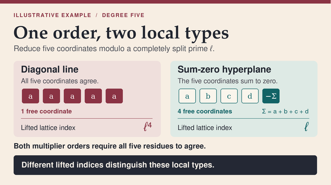
Local homothety preserves the multiplier order, but specifying that order can leave several different packets. For example, at a completely split prime in degree five, take the preimages of the diagonal line and of the hyperplane whose five coordinates sum to zero in . Each subspace projects onto every coordinate. The diagonal multipliers preserving either subspace have all five residues equal. For the hyperplane, apply a multiplier to vectors with entries and in two positions. But the preimages have indices and in . Since both span the full ring over itself, a homothety between them would have to be by a unit and preserve the index. Thus the types differ despite the common multiplier order. The theorem handles full modules, including noninvertible ones over nonmaximal orders.
5. The Proof Roadmap: Five Steps from Arithmetic to Haar Measure
The proof measures concentration indirectly. If a lattice lies in a chosen small neighborhood, a suitable one of its vectors must lie in a corresponding small box. Counting such vectors is an arithmetic problem, and upper bounds suffice to force the limiting distribution.
- Unfold the packet average. Trade repeated counts of lattice vectors along the orbits for a single sum over integral ideals. A local weight records which vectors survive the module constraints.
- Control the local weights. Calculate their exact total after weighting by reciprocal norm. Show that large local norm contributions account for very little of that total.
- Bound the ideal count. Use the zeta residue to track the scale of ideal counts. Removing primes already handled by the local weights produces an Euler factor that cancels when the pieces are recombined.
- Control the cusp and small balls. Count vectors near zero to show that the packet probabilities are tight. Count vectors near a point with no zero coordinates to bound how much of the limit can concentrate in a small ball.
- Apply entropy and rigidity. Diagonal orbit directions account for one fewer power of the ball radius than the proof gains. This surplus forces positive entropy in almost every ergodic component, where prime-degree measure classification identifies Haar.
6. Step 1: Transform Torus Packets into Weighted Ideal Counts
Saturate to the fractional -ideal , the smallest -module containing it. Write for the saturation index, for the field discriminant, and for the counting scale. The inclusion gives , so the theorem’s discriminant hypothesis forces .
Choose one fractional ideal per ideal class. The lattices in the prescribed type that saturate to are obtained by patching local unit translates of normalized modules . At primes away from there is only one choice. Lemma 2.1 shows that averaging uniformly over ideal classes and finite local labels, then integrating over a real unit fundamental domain with normalized Haar measure, gives the volume-weighted packet probability. Quotienting by the units accounts for duplicates, signs, and the actual periods.
Write for the packet probability. For a nonnegative test function , let sum its values over the nonzero vectors of a lattice. A nonzero gives an integral ideal . Its generators in this construction differ by units. Summing over those generators unfolds the unit fundamental domain, leaving an integral over vectors of absolute coordinate product , in logarithmic coordinates and all signs. With the absolute ideal norm, the product of local containment probabilities, and the residue of at one, Proposition 2.2 gives the exact identity.
The analytic class-number formula supplies the denominator through the class number and the logarithmic volume of the unit domain.
7. Step 2: Control Local Modules with Containment Probabilities
At a prime dividing , group vectors into shells indexed by their valuations at the primes of above . The local probability is the fraction of unit translates of that contain a given vector in that shell. Units act transitively on the shell, so this equals the fraction of shell volume inside . For the split diagonal-line example, when all five coordinates are units, their independently randomized nonzero residues must agree. The probability is . If exactly one coordinate is nonzero modulo , the probability is zero.
Let collect the shell indices, be the ideal norm contributed by primes over , and the product of the local zeta factors at one over those rational primes. Each normalized module has additive measure equal to the reciprocal of its index. Summing shell volumes and multiplying over primes gives Lemma 3.1’s identity.
Full span over the maximal local ring ensures that each component projection contains a unit. Its integer multiples already give many distinct residues modulo high powers of the local prime. This bounds the probability of large component valuations even when the projections are correlated. Lemma 3.1 takes a positive moment of with exponent and obtains a tail for the reciprocal-norm sum over .
8. Step 3: Bypass Subconvexity Using Stark, Shiu, and Zeta Residues
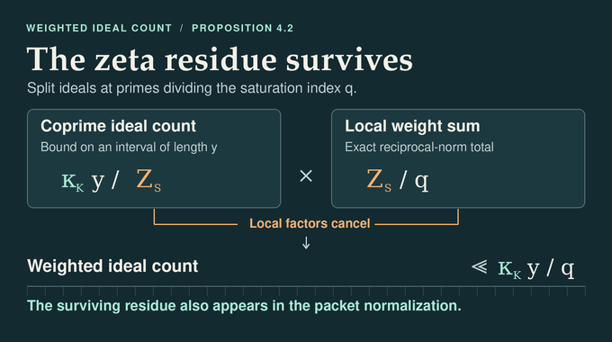
A zeta upper bound that loses track of can be too coarse after division by the packet normalization. Stark’s exceptional-zero descent says that a real zero sufficiently close to one on the scale would force a quadratic subfield. The tower law excludes such a subfield in odd degree. With this zero separation, Lemma 4.1 controls the regularized zeta function near its pole and gives for when is sufficiently large. Bounded field discriminants are handled by the simple poles of the finitely many zeta functions involved.
Split each ideal into the part supported over primes dividing and the part whose norm is coprime to . Shiu’s bound, in Pollack’s uniform formulation, controls the latter count in an interval. Removing the primes dividing divides the resulting upper bound by . Summing the local parts restores by Lemma 3.1, leaving . For large local norms, the power-saving tail absorbs the logarithmic losses of an elementary divisor bound. Proposition 4.2 gives the resulting bound.
Here and , for fixed and . The threshold for may depend on those parameters, and only enters the bound’s constant.
9. Step 4: Establish No Escape of Mass and Small-Ball Bounds
A lattice deep in the cusp has a short nonzero vector. Count vectors in a cube of radius about zero. Their absolute coordinate products are at most , so the contributing ideals have norm at most . The logarithmic fiber volume grows near small products, but the cumulative ideal bound controls this growth by integration. Proposition 5.1 bounds the limiting upper probability of a vector shorter than in the sup norm by . Mahler’s compactness criterion says that a uniform lower bound on shortest vector length keeps unimodular lattices in a compact set. This gives tightness and no escape of mass.
For a small lattice-space ball, follow one vector at its center with every coordinate nonzero. All nearby lattices carry a corresponding vector in a box of side length proportional to . The first logarithmic coordinates in this box give a factor , and the coordinate product confines the ideal norm to an interval of length . Proposition 4.2 gives the remaining factor after normalization. Proposition 5.2 then bounds the mass of an ordinary ball in any weak limit by , uniformly over centers in a fixed compact set . The packet limit is taken at each fixed radius.
10. Step 5: Convert Small-Ball Bounds into Positive Entropy and Rigidity
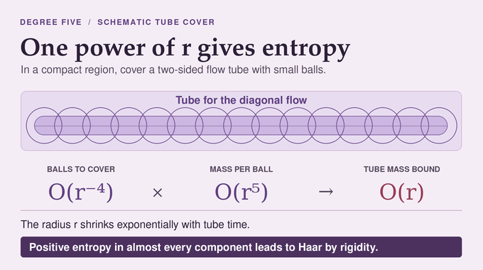
Choose a diagonal flow with distinct logarithmic speeds summing to zero. In a two-sided tube, perturbations must stay small after conjugation by both and . This squeezes every off-diagonal entry at least as fast as , where is the smallest gap between speeds. The determinant-one constraint places the diagonal part within of a matrix in . Those diagonal directions stay bounded and have dimension . Covering them takes ordinary balls of radius proportional to . In degree five, four diagonal directions consume four powers, leaving as the tube mass bound.
The ELMV tube criterion turns exponential decay into entropy at least for the time-one map, as quantified in Proposition 6.1. The ball estimate holds for any invariant probability dominated by a finite multiple of the limit. If zero-entropy ergodic components carried weight , their normalized mixture would be dominated by times the limit. Its entropy would be zero by the entropy integral formula, contradicting the tube criterion. Hence almost every diagonal-ergodic component has positive entropy. Prime-degree measure rigidity then identifies each such component with Haar probability. Tightness and uniqueness of this subsequential limit give convergence of the full sequence.
11. What the Proof Resolves and What Remains Outside Its Scope
For maximal orders, the theorem recovers equidistribution of packets built from ordinary ideal classes and sign translates as field discriminants grow. It also covers a single fixed field when the multiplier-order index grows without bound. Appendix A identifies the packet probability with the pushforward of adelic torus Haar probability, connecting the lattice description with the usual formulation using real and finite places. Individual orbits, quantitative convergence rates, and composite degrees remain outside Theorem 1.1.
OpenAI attributes its manuscript collection to an unnamed internal model. The five stages above reconstruct the written argument. OpenAI’s Lean scope note reports formalization of weak convergence and tightness for the full prime-degree statement. The public comparator specifies the target theorems and uses sorry placeholders for their proofs.
The central gain in torus packet equidistribution is keeping the zeta residue through the count. Together with the exact local normalization, it gives enough control to preserve all the mass and lets measure rigidity determine where that mass goes. Follow Binary Verse AI for more paper-first explanations of AI-generated mathematics.
What is torus packet equidistribution?
It is the weak convergence of weighted collections of compact periodic torus orbits toward an invariant probability distribution. In this paper the limiting distribution is Haar probability on the space of unimodular lattices.
How does OpenAI’s proof extend Duke’s theorem?
The paper establishes the packet form of the higher-dimensional Duke problem for totally real number fields of every fixed prime degree at least five. It covers arbitrary local homothety types as the multiplier-order discriminants tend to infinity.
Why could previous methods not establish this full result?
Earlier approaches depended on estimates such as subconvexity or imposed restrictions on fields, orders, or local structures. The new argument gets the required upper bounds from weighted ideal counts that retain the Dedekind zeta residue.
Why are arbitrary local homothety types important?
They allow the theorem to cover full lattices with different local module structures, including noninvertible modules over nonmaximal orders. Several distinct local types can share a multiplier order, so that order alone may describe several packets.
How does the proof obtain positive entropy?
The proof bounds small-ball mass by on compact sets. Covering a two-sided tube along the diagonal directions leaves an exponentially decaying mass bound. Applying the entropy criterion to normalized mixtures of components shows that almost every ergodic component has positive entropy.
What does no escape of mass mean?
The packet probabilities stay tight as the discriminants grow. For any prescribed mass error, a compact part of the lattice space contains all but that amount of mass for sufficiently large discriminants. The limiting measure therefore has total mass one.
Does the theorem prove that every individual torus orbit equidistributes?
The theorem concerns complete, volume-weighted packets. It leaves individual-orbit convergence, a quantitative convergence rate, and composite degrees outside its scope.