
A zeta zero off the critical line would leave a trace in the primes. How much of the prime count would you need to rule it out? Levent Alpöge’s Riemann Hypothesis proof with Claude takes that route. Successive theta lifts supply arithmetic data for a smoothed prime-power sum, and a Landau argument shows that a zero to the right of one-half would force derivatives larger than those estimates permit. The functional equation then excludes the left side. Alpöge’s four-page announcement, released November 20, 2026, gives the discovery outline. The released Lean archive, beginning with part one formalizes RH and Dirichlet GRH. Andrew Sutherland’s verification report records successful checks by independent kernels.
Table of Contents
1. The Riemann Hypothesis: What Must Actually Be Proved?
Write with . Absolute convergence and unique factorization give the product over primes .
Analytic continuation extends zeta meromorphically, with a simple pole at and trivial zeros at the negative even integers. The other zeros lie in the critical strip . RH places each on . In explicit formulas, a zero contributes a term of scale , with oscillation if , in weighted prime counts. A Dirichlet character modulo weights integers multiplicatively by residue class, taking value zero on nonunits. Inserting in the series defines for . Characters let explicit formulas distinguish prime counts in different residue classes. The modulus-one character recovers zeta.
2. Why Earlier Methods Stop Short of the Critical Line
The Euler product excludes zeros for . Classical zero-free regions cross , but the guaranteed strip near that boundary narrows at large height. They leave points with unaccounted for. A lower bound for the proportion on the line still permits exceptions, as does the proposed fixed zero-free region ending at 7/8.
Over finite fields, Stepanov’s method constructs an auxiliary function that vanishes to high order at rational points of a curve. A divisor counts those zeros with multiplicity. If every point contributes at least to the degree of the zero divisor, the degree budget bounds the point count after division by . At a smooth point, vanishing of the first coefficients in a local parameter imposes exactly that order. Primes do not supply the same local-parameter construction. Alpöge’s route seeks a comparable gain through automorphic data.
3. The Riemann Hypothesis Proof Strategy in Six Stages
- Chain theta lifts so that successive transfers contribute arithmetic constraints, playing the part of repeated vanishing.
- Choose windows where local-to-global cohomology costs stay within budget for fields adapted to the target character.
- Match theta periods in a common space. Use integral lattices and their norms to turn divisibility and period estimates into a size comparison.
- Convert that comparison into a signed bound for corrected prime-power sums. Balance the lift costs to reach the square-root exponent up to a small loss.
- Use high derivatives of a Mellin transform to detect a pole that any forbidden zero would create. The window bound makes that pole impossible.
- Extend nonvanishing to all moduli and use the functional equation to reflect a hypothetical left-side zero into the excluded half-plane.
Here is a weighted family of characters, controls the exponent loss, and denotes a nontrivial zero. The nonvanishing statement sets aside the pole of a principal character at .
4. Theta Lifts: Replacing Multiplicity With an Automorphic Chain
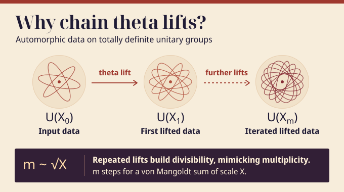
A theta lift transfers automorphic data between groups paired through the Weil representation. One integrates a theta kernel against input automorphic data on one group to obtain an output on the other. The announcement describes iteration along unitary groups that are definite at every archimedean place. In its schematic parameter bookkeeping, a step adjoins a block built from a character to the input parameter. That permits another step with fresh data, accumulating divisibility through the chain of lifts.
A model determinant shows the point. If column of an integral matrix is divisible by , its determinant is divisible by . A bound on the column norms limits the absolute determinant. The chain must accumulate divisibility and still leave enough independent directions for a useful comparison. Alpöge traces the idea to Fourier analysis in a toy setting and credits Claude with proposing chain length for a sum of scale .
5. Galois Representations and the Local-to-Global Arithmetic Argument
Over a CM field, a totally imaginary quadratic extension of a totally real field, the construction associates -adic Galois representations to regular algebraic cuspidal automorphic data under polarization hypotheses. Traces and characteristic polynomials let the proof compare local Galois and Langlands data. Geometry supplies initial representations; congruences, limits of traces, descent and theta lifting extend the construction. Frobenius and monodromy comparisons have separate local hypotheses.
A key cost comes from cohomology classes unramified outside that restrict to zero at every place above . The coefficients are -power torsion with a negative Tate twist. Taking the kernel of restriction isolates global classes invisible to those local tests. Its finite module length, multiplied by , is its logarithmic size. For generic primes, trace congruences bound the lengths by valuations of integers shared across coefficient primes. Unique factorization then bounds the total. The Iwasawa-theoretic part handles exceptional primes by selecting intervals where problematic twists within range have a cheaper bound. The window theorem fixes the target character and tolerance first, then gives an entire late interval for the aggregate bound across eligible fields and twists. These estimates supply a cohomology budget that the lattice comparison can absorb.
6. Theta Correspondence, Seesaw Identities, and Matching Conditions
A formal integral produces a useful lift only with convergence and appropriate local data. In the matched theta models, test vectors from distinct spaces map into common local representations, with fixed unramified vectors away from the exceptional places. The agreement theorem relates the global integrals by a nonzero scalar for the prescribed data. Lift existence supplies the representations along the chain; matching makes the test data comparable.
A seesaw identity moves a lift across a period pairing and expresses the periods through Bessel pairings in a common target. This makes period maps and their scalar normalizations comparable across characters. To see what averaging buys, let denote normalized period maps into a target of dimension , and set . If and , Cauchy–Schwarz on the nonzero eigenvalues gives . Small therefore forces the images to span nearly the whole target. The proof transports these maps and their norm estimates to the same integral lattices used for the arithmetic bounds.
7. Divisibility, Lattice Slopes, and Covolume Estimates
Finite-place congruences and divisibility let the proof rescale the source lattices while keeping their period maps integral. At infinity, a Bost-type slope comparison bounds how much size can be lost in passing from the sources to the target. In the Euclidean model, mean slope is minus the logarithm of covolume divided by rank. Scaling every basis vector by increases the log covolume by the rank times and drops the slope by .
The comparison retains good directions and bounds the loss from the bad directions by controlling both their rank fraction and their maximal slope. Clearing the denominators of the projection costs additional logarithmic size. Arithmetic Hilbert–Samuel estimates, height bounds and descent supply the geometric covolume input. Putting the CM periods and archimedean count on the same field scale cancels their large common terms. The remaining main term matches the one subtracted from the prime sum.
8. From Von Mangoldt Sums to the Square-Root Error Bound
Let for and zero elsewhere. Put . The ramp makes a prime power enter continuously. For example, contributes once .
For zeta, define , where is Euler’s constant. For nonprincipal characters use . The comparison fixes a finite family with containing the target primitive character and uses . The family admits only the modulus-one principal character.
Finite Fourier inversion expands arithmetic class indicators in characters, with inertia averaging at ramified primes. Local divisibility contributes the same ramps after rescaling, and logarithms of prime ideal norms supply the prime logarithms. Subtracting the matched main term and averaging over translates leaves the positive-weight family. After normalization the principal competing costs behave like and , up to small powers of . At , the simplified balance puts both at when . The full comparison controls the other costs and proves
The loss exponents are fixed before . For any candidate real part , choose and then small enough to make the displayed exponent at most . The comparison holds throughout arbitrarily late windows . The target family stays fixed as the intervals move.
9. The Landau Argument: How Prime-Sum Bounds Exclude Zeros
Start with for , where a crude quadratic growth bound suffices. Integrating a single ramp gives for . Summing those integrals and logarithmically differentiating the Euler product gives the uncorrected transform for an individual character.
The corrections remove the singularity at . For a nonprincipal character the combined numerator vanishes there; for zeta the two corrections cancel the double and simple pole terms from the Laurent expansion. The real part in pairs each character with its inverse at half the original weight. If has a zero of order at , its logarithmic derivative has residue . Thus each contributing zero has residue proportional to the same factor in . Positive weights ensure a genuine pole. At a real zero in the residue itself is positive.
Put , , and take normalized derivatives at . With , differentiation under the integral and the triangle inequality give
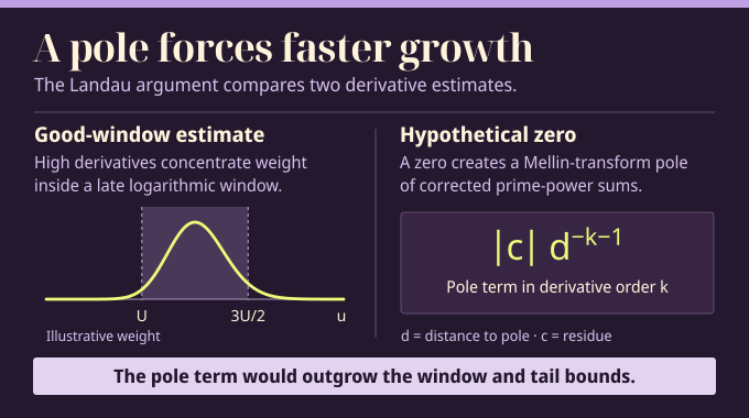
The real-center term eliminates any need to bound the negative part on a good window. Its logarithmic interval is , where . Choose with sufficiently large. The kernel peaks near . Even after paying for the global bound, the tail kernel peaks inside the interval. Exponential bounds for the two gamma-integral tails give a constant times ; on the interval the sharper bound gives a constant times for any fixed and sufficiently large .
A pole at distance from a suitable center yields a derivative term of size , where is its residue. Cauchy estimates bound the holomorphic remainder with a larger radius. For a closer pole at a shifted center, the real-center term is controlled by a larger pole-free disc. If the first pole encountered on expanding the real-center disc is real and uniquely nearest, its positive residue supplies the lower bound at the real center. Choosing below the resulting logarithmic gap between radii makes the pole term grow faster than the window bound along the selected orders. This contradiction excludes zeros with real part above . The earlier choice of excludes the candidate, and classical nonvanishing on and to the right of covers the rest, with the zeta pole excepted.
10. From Primitive Characters to Universal Dirichlet Nonvanishing
Let modulo be induced by the primitive character of conductor . Induction removes Euler factors at additional primes dividing .
When , the subtracted term in each factor has modulus at most . These factors add no zeros in the open strip. Primitive nonvanishing therefore extends to every modulus for , with excluded for principal characters.
11. The Final Deduction: Why Every Nontrivial Zero Lies on the Critical Line
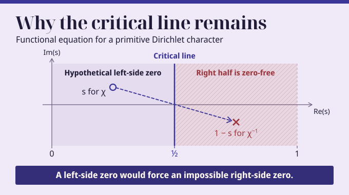
For primitive , set for even parity and for odd parity. The completed function is . Its completion factor is finite and nonzero throughout the open strip. The functional equation gives , where is the root number. If a zero had real part below one-half in the strip, the inverse character would have a zero at with real part above one-half. Right-half nonvanishing excludes both possibilities, leaving . The Euler factors extend the conclusion to imprimitive characters, and modulus one gives RH.
Lean’s Main.lean exports Mathlib’s RiemannHypothesis, a second zeta formulation, LFunction_ne_zero_of_half_lt_re, and critical-strip statements for primitive and general Dirichlet characters. The zeta declarations explicitly exclude the negative even integers and . The Dirichlet statements give the scope of this generalized Riemann Hypothesis proof. Alpöge describes extended RH for broader number-field zeta functions as a future goal.
Sutherland reports compilation, dependence on the standard axioms propext, Classical.choice and Quot.sound, and acceptance of the export by nanoda and con-leche, with independent statement matching for all five theorems. The geometric and arithmetic inputs still need a detailed written exposition. The Riemann Hypothesis proof hinges on how much information a good window preserves. Its one-sided estimate suffices because a single forbidden zero forces faster derivative growth. Follow Binary Verse AI for technical analysis grounded in primary sources.
What is the key new idea in Alpöge’s Riemann Hypothesis proof?
The construction chains theta lifts between totally definite unitary groups to emulate the gain from multiplicity in Stepanov’s function-field method. The resulting divisibility and period comparisons feed the bounds on corrected prime-power sums used for nonvanishing.
Why does the proof use approximately √X theta lifts?
At prime-sum scale , two leading normalized costs behave roughly as and , where is the number of lifts. Balancing them gives . The complete comparison also controls other costs and small exponent losses.
How do the prime-sum estimates rule out zeros?
A zero creates a genuine pole in the Mellin transform of the positively weighted family of corrected sums. A Landau argument uses high derivatives to localize to controlled intervals. A pole to the right of the chosen exponent would force growth faster than the interval and tail estimates permit.
Why does nonvanishing to the right of 1/2 prove the Riemann Hypothesis?
The functional equation takes a strip zero at to a zero at for the inverse primitive character; zeta is its own counterpart. A left-side zero would reflect into the zero-free right half. Thus all nontrivial zeta zeros lie on the critical line.
Does the proof also establish the Generalized Riemann Hypothesis?
The released and independently checked statements place every Dirichlet L-function zero in the open critical strip on the critical line. This is Dirichlet GRH. Alpöge presents the extension to broader number-field zeta functions as a future goal.
What does the Lean verification establish, and what remains to be explained?
Andrew Sutherland’s report records error-free compilation, dependence on Lean’s three standard axioms, acceptance by independently written kernels, and independent matching to all five challenge statements. A human-readable account still needs to unpack the deepest geometric and arithmetic dependencies.