
The primes 7 and 31 both leave squarefree numbers behind them. Yet 6 has two prime factors and 30 has three. Do prime predecessors like 6 keep turning up, with an even number of prime factors and no repeats? OpenAI’s September 17, 2026 preprint proves that infinitely many do. Its Theorem 1.1 says that there are infinitely many primes with . The proof builds a weighted family in which the predecessor already has even parity, then shows that composites and repeated factors cannot account for all the surviving weight.
Table of Contents
1. Prime Predecessors: What OpenAI’s Theorem Actually Proves
A prime predecessor is the integer immediately before a prime , namely . The function counts the prime factors of with multiplicity, while counts distinct prime factors. If is squarefree, meaning no prime square divides it, the two counts agree and the Möbius function is . Otherwise . The same witnesses work under either convention.
For odd primes, the squarefree condition also forces . Otherwise would divide the predecessor. The proof builds that restriction in from the start by writing with odd.
2. Why the Prime-Factor Parity Problem Resisted Classical Sieve Theory
Divisibility tests tell a sieve which small primes divide an integer. After ruling those out, it can still face a candidate that is either prime or a product of two large primes. The Liouville function separates these two cases. The parity problem in sieve theory is that the usual counts of multiples, even when accurate on average, can be compatible with different distributions of the two Liouville signs. Friedlander and Iwaniec’s asymptotic sieve illustrates what additional bilinear information can buy.
Earlier work on smooth shifted primes by Baker and Harman and by Lichtman put bounds on how large the prime factors of can be. That controls factor size. Here the sieve must preserve the preselected parity while detecting primes. A ceiling on factor size leaves both parities possible.
3. The Proof Strategy: From p = 2u + 1 to Infinitely Many Primes
- Build the parity into the candidates. Assemble odd integers from prime factors in prescribed size bands. Keep the ones with odd total multiplicity, so doubling each candidate gives even parity.
- Make the long prime sum cancel. Prove a uniform bound on an oscillatory sum over the prime in one designated factor slot. This gives the correlation argument control at high frequencies.
- Keep the sign in shifted correlations. Lift a pair of nearby arguments to the dilation graph. They pick up the same sign from their shared multiplier, whose square is one.
- Turn the correlation into distribution. Write a prospective prime as a product of two factors. Comparing two representations produces a shifted correlation of the controlled kind. This gives a way to replace sensitive tests on a factor by local averages.
- Leave positive mass for primes. Presieve by congruences, use those replacements to bound composite contributions, and discard predecessors with repeated prime factors. A positive remainder at arbitrarily large scales proves infinitude.
OpenAI attributes the release’s results to an internal frontier model. The repository’s published reasoning summaries cover other results in the release. The roadmap follows the manuscript’s proof dependencies.
4. Constructing Nonnegative Weights That Select Odd Prime-Factor Parity
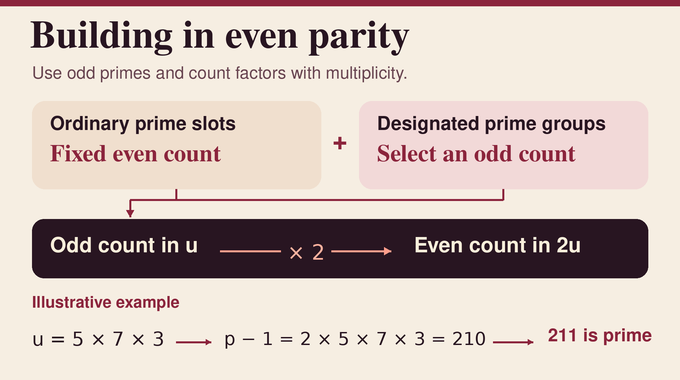
Section 5 separates the allowed primes into ordinary bands and disjoint groups . Write for their union, for the part outside it, and for the exponent of in . Each ordinary band contributes a fixed even number of prime slots. Its weighted tuple count contributes to . The marking weight requires a divisor from each group and damps contributions from integers with many distinct group divisors.
The projection is one for odd group-prime multiplicity and zero for even multiplicity. Because the ordinary slots contribute an even count, positive weight forces to be odd. Every allowed prime is odd, so doubling adds exactly one factor of 2. Write for the total weight in the window selected by the smooth cutoff , supported on . Repeats are allowed during construction. Lemma 5.3 bounds their eventual cost by : under reciprocal weighting, collisions between ordinary slots are rare, and an occurring group prime repeats with conditional probability under the group harmonic measure.
The localization itself uses a free slot in the highest ordinary band. With the other large slots near their band midpoints and the group product restricted in size, the free prime can place where is positive. The prime number theorem gives reciprocal prime mass of order for that slot, with . Lemma 5.2 thus gives for a fixed constant . This makes the later logarithmic error estimates meaningful relative to the candidate mass.
5. Long Prime Dirichlet Polynomials and the New Cancellation Estimate
The designated slot has a prime ranging over a positive-power scale in . Once Fourier analysis introduces the logarithmic phase , the proof needs cancellation between the resulting complex terms. Write . Lemma 3.1 gives the following bound for every fixed and . Uniformly for intervals with , characters modulo for fixed , and , it bounds the prime sum below. The exponent depends on the fixed data.
Here denotes an upper bound up to a constant factor. The starting point is a count of pairs of tuples whose sums of like powers agree through degree . Lemma 3.2 iterates a congruence argument that shortens the variable range and shrinks the exponent loss by a factor per step. Controlling the constants matters because the logarithmic phase is approximated on short blocks by Taylor polynomials whose degree can grow with . The resulting cancellation for sums over ordinary integers in progressions bounds Dirichlet -functions in a narrow strip around the line .
A local expansion of the logarithmic derivative isolates nearby zeros. Positivity from the Euler products rules out a zero too close to the line, giving a zero-free strip of width to the left of that line at the heights used. After smoothing the interval, Mellin inversion writes the von Mangoldt weighted sum as an integral involving the logarithmic derivative of the -function. Moving left inside the strip supplies a factor . This beats every fixed inverse power of after the remaining costs. Removing higher prime powers and the factor gives the prime estimate for the next stage.
6. The Common-Sign Cancellation That Preserves Parity
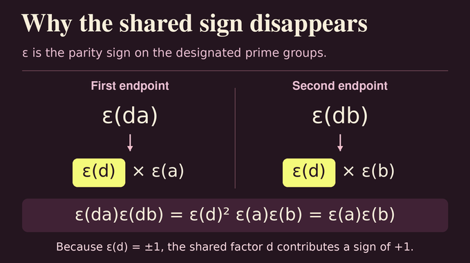
Theorem 4.1 controls weighted correlations of two structured sequences at and , for nonzero integer bounded by a fixed power of . Both endpoints have a designated prime slot and may carry the same twist , chosen to be either the constant one or the group-prime sign . The two choices are needed because the parity projection in is a difference of unsigned and signed weights.
The graph represents the endpoints using a shared factor made of group primes. Removing it leaves arguments and and preserves the part of each endpoint supported outside the groups. Complete multiplicativity gives even when a prime in also divides . The shared sign occurs twice.
Thus removing the dilation leaves the reduced endpoint signs intact. The graph controls the combined pairing. Isolating the raw correlation requires bounding each comparison.
7. Weighted Dilation Graphs and the Control of Shifted Correlations
In the companion paper’s construction, a physical graph state records an integer and ordered lists of marked group-prime divisors. A transition shifts the integer by a multiple of a product of prime labels. The ideal operator models the corresponding label draws probabilistically. The companion paper proves that a residual operator, consisting of the original transition plus signed comparisons, has small ideal norm. Its transference theorem carries that control to the actual weighted integer pairing.
The raw transition becomes the required shift after removing the shared dilation. To isolate it, the manuscript must bound the comparisons separately. Each comparison frees independent products of prime labels from two blocks of large groups. Their product supplies a bilinear Fourier multiplier. It is small on the minor arcs, where additive frequencies are away from the relevant rational neighborhoods. Parseval then controls this part of the comparison sum. On the major arcs, the argument bounds local Fourier energy using Dirichlet polynomials.
A small-prime polynomial restricts the difficult frequencies to a sparse set. At the large exceptional frequencies, Lemma 3.1 controls the long prime polynomial. At the small ones, the first endpoint’s coefficients are assumed to have small sums against over intervals, for characters of small modulus and bounded frequencies. This is the character–Mellin discrepancy condition. No such condition is imposed on the second endpoint. Bounding and subtracting the comparisons leaves the twisted correlation estimate.
8. Type II Bilinear Distribution: Turning Correlation Bounds Into Sieve Power
Theorem 6.1 tests the weights along with coefficients and bounded by a fixed power of . The factors occupy intervals inside dyadic ranges of scales and , with and each scale between and for fixed . Only needs the discrepancy bound and rough support, meaning its supported integers have no prime factor at or below the cutoff . Under these hypotheses the bilinear sum is small for any fixed target saving .
To see where the shift comes from, split by smoothly allocating ordinary slots, keeping the designated prime and group-prime part in . The factor stays within logarithmic powers of , with an upper scale deliberately below . Fourier inversion separates the allocation into coefficient factors. Cauchy–Schwarz then compares two representations and with fixed. Divisor moment bounds handle the diagonal, aided by the reduced scale of .
Off the diagonal the differences are and . Set . The second endpoint is , because . The lower bound on keeps within a logarithmic power. Rough support keeps group primes out of and , so the signs on become exactly the signs on . Theorem 4.1 now applies to the correlations produced by the square. Type II can then compare a primality or roughness test with a local average.
9. Congruence Distribution and Local-Density Approximations
For odd squarefree , the condition chooses the single unit residue . The predicted weight is , where is Euler’s totient function. Theorem 7.1 bounds the sum of absolute errors over such by for fixed and . The manuscript separates an ordinary prime from its highest band and uses Siegel–Walfisz estimates for small conductors and the multiplicative large sieve for larger ones. This averaged control makes the block sieve’s remainder small.
The local proxies have a different job. In each short cell on the logarithmic axis, divide the number of integers passing the desired test by the number that are -rough. The proxy takes this ratio on rough integers and zero elsewhere. The imported discrepancy estimates apply even on intervals that cut across a cell, with the ratio still computed on the full cell. The resulting coefficients stay between zero and one, so the paper can increase their precision after fixing the discrepancy demanded by Type II.
10. Prime Extraction: Eliminating Semiprimes and Proving Infinitude
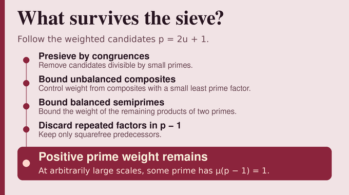
Write . A block sieve first keeps the weight for which avoids primes up to , with small and fixed. For an unbalanced composite, the least prime factor lies above this threshold but at most . The complementary factor has no prime divisor below , including when divides it again. In logarithmic bins for , Type II replaces the roughness test on with its proxy. A conditional sieve supplies the weight for each bin. The companion paper’s rough-number density integral counts by the least prime and reserves a unit term for primes. This margin leaves at least for primes and balanced composites together, with a fixed local-density constant.
A remaining composite has exactly two prime factors counted with multiplicity: three factors above would exceed for the chosen small . The proof replaces both prime indicators, one at a time, by bounded proxies. A positive sieve bound controls rough pairs near . There are dyadic scales for the first factor and only a bounded number for its partner at each scale. The prime proxies contribute reciprocal logarithmic factors, and the rough-pair bound cancels their rough-density normalizations. The semiprimes cost at most , with fixed before choosing . Choosing so that leaves prime weight comparable from below to .
Finally, the weight lost to repeated factors divided by tends to zero. For every sufficiently large scale, some supported therefore gives a prime with squarefree predecessor and even parity. Those primes grow without bound.
11. What OpenAI’s Prime-Predecessor Proof Establishes and Its Limits
The result is an infinitude theorem for squarefree prime predecessors of positive Möbius sign. The manuscript gives neither a natural-density asymptotic nor an effective threshold for the construction. The release announcement discusses Lean formalizations across the collection. The evidence for the result described here is the written preprint and its stated dependencies.
The proof preserves parity until it can separate prime weight from composite weight. That is a route through the sieve obstruction for this specific family of prime predecessors. Follow Binary Verse AI for independent, source-based analysis of AI-assisted mathematics.
What does OpenAI’s prime-predecessor theorem prove?
It establishes that infinitely many primes have a squarefree predecessor with an even number of prime factors. Equivalently, for infinitely many primes.
Why does the Möbius function equal 1 for these primes?
For a squarefree integer , the Möbius function is , where counts distinct prime factors. An even count gives . If a prime square divides , then .
Why couldn’t classical sieve theory establish this parity result?
Classical sieve methods primarily use counts of multiples. Those counts can be consistent with different proportions of integers having an even or odd number of prime factors. The proof adds shifted-correlation and bilinear estimates that give it information beyond the divisibility counts.
What is the central mathematical innovation in OpenAI’s proof?
The proof establishes a cancellation estimate for a long sum over primes and extends the shifted-correlation argument to carry the same parity sign at both endpoints. Complete multiplicativity makes the sign of their shared dilation appear twice, so its contribution is one.
Why are weighted dilation graphs necessary?
They transfer operator bounds on a model of the prime labels to correlations of the weighted integers. The prime-slot estimate and parity-twist identity then help isolate the shifted correlation needed for Type II distribution.
How does the proof distinguish genuine primes from semiprimes?
The extraction argument bounds the weight of unbalanced composites after presieving. Any surviving composite has exactly two prime factors counted with multiplicity. The proof bounds their weight as well, leaving positive weight for genuine primes.
Does the proof establish that half of all primes have squarefree predecessors with even parity?
No. The theorem establishes infinitude. It gives neither a natural-density asymptotic for the qualifying primes nor an effective threshold at which the construction must produce them.