
Take the integers 2, 3, and 4. Each shares a prime factor with 6. You need a fourth slot to guarantee a coprime integer wherever the interval starts. How long can that run get with primes? OpenAI’s Jacobsthal function proof shows that for every integer , the worst-case interval length is at most for one absolute constant . The guarantee holds for every starting point and every positive modulus with at most distinct prime factors. The result answers Jacobsthal’s quadratic-bound question and gains a squared iterated logarithm. The proof reaches the point where the leading linear-sieve lower bound vanishes, then shows that a smaller positive contribution survives in the actual integer count.
Table of Contents
1. Jacobsthal Function and OpenAI’s Quadratic-Bound Theorem
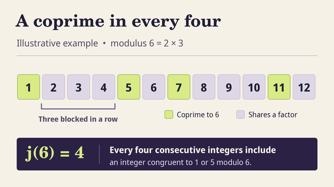
For a positive integer , the Jacobsthal function is the least length for which every interval of that length contains an integer coprime to . Write for its number of distinct prime divisors. The worst-case function is the maximum of over positive integers with . In the example above, the coprime residues modulo 6 are 1 and 5. Their successive spacings are 4 and 2, repeating, so every four consecutive integers contain one and .
Theorem 1.1 in OpenAI’s September 25, 2026 preprint gives the bound below. All logarithms are natural.
2. The Original Jacobsthal Question and Why Earlier Bounds Fell Short
A prime can cover one residue class at a time. Prime powers give it no additional coverage because coprimality depends only on which primes divide the modulus. The longest fully covered interval has length . Allowing exactly primes gives the same maximum since adding prime factors can only extend the set of covered integers. Erdős recorded Jacobsthal’s question about a uniform quadratic upper bound, catalogued as Erdős Problem 970.
Erdős noted that Brun’s method gave a polynomial bound for an absolute exponent . Vaughan obtained the uniform bound for . Iwaniec had obtained the scale for the first primes. His later shifted-sieve argument reached that scale for arbitrary prime sets, cutting two logarithmic factors from Vaughan’s bound. Here and below, means bounded above up to a constant.
3. Proof Roadmap From Forbidden Residue Classes to a Quadratic Bound
- Turn the gap into a covering problem. Translate the interval into coordinates starting at 1. Each divisor prime forbids one congruence class. First handle every prime up to a chosen cutoff, and aim to leave a reserve of integers.
- Build a reference sieve. Sort the excluded integers by their first forbidden hit. Repeat inside progressions. Replace each small-prime count by its density prediction.
- Recover the boundary contribution. Follow the reference tree down to small exponents. A renewal calculation aggregates the boundary terms with their signs and proves that the normalized root count is positive.
- Compare with actual counts. Locate large errors on individual edges. Many such errors imply rational alignment. Variance estimates and exact counts at selected even nodes keep these errors from using up the reference margin.
- Account for the remaining divisor primes. Each large prime removes only a bounded share of the reserve. Choose the cutoff so the total loss leaves at least one coprime integer.
OpenAI’s release attributes the collection’s results to an internal frontier model. These stages reconstruct the manuscript’s argument. The announcement gives collection-level information on how the results were obtained.
4. The Linear Sieve Barrier at the Critical Parameter
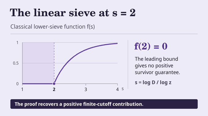
The classical linear sieve compares its modulus level with its prime cutoff through . Each intersection counts a residue class modulo a prime product. The level must keep the accumulated endpoint errors under control. At interval length , even choosing on the scale of gives tending to 2 from below. The paper’s tree has its own root ratio, which also approaches 2 from below.
The lower and upper functions and govern the leading sieve bounds. In the paper’s normalization, for , and for , where is Euler’s constant. Just above 2, through . The leading lower bound disappears at 2, leaving finite-cutoff terms to examine.
5. The Uniform Covering Estimate and Its Survivor Count
The Chinese remainder theorem gives a common shift satisfying for each prescribed class . Avoiding the classes is therefore equivalent to being coprime to the product of the primes. For instance, forbidding the even class and the class 1 modulo 3 makes the forbidden positions . The survivors are 3 and 5 modulo 6, exactly the classes coprime to 6 after subtracting 4.
For a sufficiently large real cutoff , put and . Sieve the small primes up to inside progressions. The primes in build the tree. Define and , the small-prime density. Let be the number of survivors in . Theorem 1.2 guarantees an absolute such that every assignment of classes gives
Mertens’ theorem gives , where means the ratio tends to 1. A guarantee of one survivor could be erased by a single additional prime. This quantitative reserve makes the final step possible.
6. The Decreasing-Prime Tree and Its Admission Rules
At a node with prime product , let count integers that hit every prescribed class for primes dividing and avoid the classes at primes up to . Let also require avoiding the available primes above up to the node’s cutoff, strict after the root. For a prime , write . Assign each discarded integer to its smallest available forbidden hit. Its child must avoid every smaller available hit, giving equation (3.2).
This makes the cutoffs decrease. Subtraction reverses the bound at each depth, so even nodes are lower nodes and odd nodes are upper nodes. An even node admits every available child. An odd node can omit a nonnegative child from its subtraction and still give an upper bound. It admits a child of exponent only if , where and . This keeps included progressions long enough for a uniform upper sieve. Stopping instead replaces an already admitted even subtree by its exact count.
The reference count shrinks by on an edge, so the reference expansion assigns each path harmonic weight .
7. Recovering the Boundary Contribution With Delay Functions
Delay equations link the two classical functions. The lower equation holds for , and the upper equation holds for . The shift by one corresponds to spending one cutoff unit when forming a child at the current cutoff. The paper continues the logarithmic formula for just below 2 at the starting lower state. With , the continued root benchmark contributes after multiplication by the reference density above .
The low end of the tree behaves differently. Its exponents start at 1, and the extra admission constraint matters below exponent 2. At cutoff 2, the proof compares the finite reference polynomial with its classical benchmark for each parity. These boundary discrepancies have signs and decay rapidly for large remaining gap. For example, at odd gap 2 and cutoff 2, no lower child passes admission. The normalized reference value there is 1, while the limiting benchmark is . The negative discrepancy enters positively at odd depth. Its contribution still has to be combined with those from other states. The Dickman function gives the decay of the difference between the upper and lower functions, while the Buchstab function gives their sum after normalization. Together they identify the benchmark and bound its deviations.
8. Harmonic Paths, Regeneration, and Renewal Theory
Replace reciprocal-prime sums by integrals with measure . Positive derivative weights and turn the continuous tree with the ratio constraint into an alternating probability process on , where is the remaining gap. A child with exponent has ratio . The harmonic step becomes after reversing the limits. The change of measure telescopes. Converting a path probability back to harmonic mass introduces a squared endpoint-to-starting gap ratio and a ratio of derivative weights. Compact endpoint ranges therefore contribute at scale .
When an odd state has ratio at most 3, its next draw has the same distribution throughout that range. These returns split the process into independent, identically distributed cycles. The gap decreases multiplicatively, so its logarithmic decrements add. Renewal theory gives the limiting occupation of fixed log-gap windows, using different invariant densities for even and odd states. The parity matters because even and odd boundary terms enter with opposite signs.
The paper couples this process to prime paths using estimates for reciprocal-prime sums in short bins. Tail and quadrature bounds justify transferring the signed integral. Proposition 6.3 proves that converges to a value greater than , where is the even reference value divided by its node density prediction. This includes the negative root contribution and the admission losses.
9. Inverse Estimates for Discrepancies in Actual Residue Classes
Long progression counts are close to by the fundamental lemma of the sieve. At a short endpoint, a large discrepancy must be visible within the last few edges, where the child count differs sufficiently from the parent count divided by the new prime. The paper groups regular paths into boxes of short prime bins. An isolated earlier prime and the prime on the witnessing edge can vary independently inside the full box.
The inverse estimate runs from unusual counts back to arithmetic structure. The additive large sieve bounds how often such biased residue tests can occur across edge primes. If too many witnessing edges lack a structured explanation, the incidence constraints give many integer points with too few permissible slopes. Small-height polynomial interpolation produces a curve through those points. Convex-arc lattice-point estimates bound the contribution of nonlinear components, and a larger-sieve pair count helps constrain the rational alignments. Outside a small exceptional fraction, a witnessed error comes with a rational from a list fixed for the box. An aligned prime satisfies .
First and second moments for small-prime survival, with uniform estimates as the isolated prime varies, make large errors rare when the effective modulus or scaled intercept is large. The persistent exceptions have small effective size, and their sufficiently large path primes align to the same rational.
10. Stopping Exceptional Branches and Completing the Proof
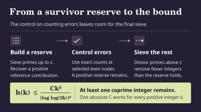
The proof looks for bins where almost all primes align with one eligible rational. It tags an aligned prefix and stops at the first qualifying even node in a prescribed window, with enough admission slack to vary the tag prime. A marked-renewal argument shows that almost all the remaining exceptional mass passes through such stops. Averaging exact survivor counts over the aligned choices of the tag prime covers the reference subtree values in aggregate.
For expanded nodes and stops , let be the root reference value and the stopped lower bound. Equation (3.7) becomes
Here is the cutoff at node . The first sum is controlled in absolute value by separating long progressions, small relative errors, and the few bad endpoints left outside stopped subtrees. Together these cost at most three eighths of the guaranteed reference margin. The second sum is nonnegative by the stop comparison. This proves Theorem 1.2.
For Theorem 1.1, choose , with a sufficiently large fixed constant. Prescribe the divisor classes in the translated interval and arbitrary classes at the other primes up to . Put . Each remaining divisor prime hits at most positions on one progression. A smaller upper sieve bounds the survivors it can remove by . Summed over at most primes, the loss has coefficient proportional to relative to the reserve. A coprime integer remains in the interval, of length . Elementary inclusion-exclusion handles the finitely many smaller : the density of coprime residues is at least and the total endpoint error is at most .
11. What the Quadratic Bound Resolves and What Remains Open
Let be the primorial, the product of the first primes. Hajdu and Saradha found , disproving Jacobsthal’s separate primorial extremality conjecture. Primorials still provide lower bounds. The same covering constructions produce large gaps between consecutive primes. The long covered intervals of Ford, Green, Konyagin, Maynard, and Tao give as tends to infinity. The symbol denotes a lower bound up to a positive constant. The gap between the upper and lower scales leaves the true growth rate open.
The preprint leaves unspecified, so the asymptotic estimate supplies no explicit numerical ceiling for an individual . The pinned Lean conclusion states the quadratic theorem. The repository’s formalization scope notes separately report the strengthened iterated-logarithm bound, with arbitrary signed interval starts.
The Jacobsthal function now has a uniform upper bound below the quadratic scale. The proof’s decisive step is to retain enough of the finite boundary term to pay for actual counting errors and the remaining divisor primes. Follow Binary Verse AI for more research explainers that trace the argument from the original question to the theorem.
What did OpenAI prove about Jacobsthal’s function?
OpenAI proved for every integer , with one absolute implied constant. This gives a uniform bound for every positive modulus with at most distinct prime factors and for every interval starting point.
Why did the classical linear sieve fail to establish the quadratic bound?
At the critical sieve parameter , the classical lower-sieve function satisfies . The leading estimate gives no positive lower bound there. The proof recovers a smaller positive boundary contribution and controls the discrepancy between the reference calculation and the actual counts.
What is the key mathematical innovation in OpenAI’s proof?
The proof uses a decreasing-prime tree and renewal theory to establish a positive reference margin. Inverse estimates and variance bounds identify the difficult residue-class configurations, and exact counts at selected even nodes preserve the margin in the actual sieve.
Does the proof show that primorials always maximize Jacobsthal’s function?
That separate conjecture is false. The paper cites and , where is the product of the first 24 primes. The new upper bound applies to arbitrary prime sets.
Does the quadratic-bound proof determine the exact growth of Jacobsthal’s function?
The exact growth of the worst-case function remains open. The theorem improves the uniform upper bound, and a substantial gap remains between the established upper and lower bounds.
Can the new theorem calculate an explicit maximum gap for a given number of prime factors?
The theorem establishes the existence of one absolute constant and leaves its value unspecified. It therefore gives an asymptotic upper bound without calculating the exact worst-case gap for a given .