

A prime desert is easy to admire and surprisingly difficult to count. One enormous gap can contain thousands of empty intervals, making rare events look common. OpenAI’s September 25, 2026 manuscript, Positive Lower Density of Large Prime Gaps, presents a proof that large prime gaps occur with positive lower density: for every fixed positive multiplier, a positive proportion of consecutive gaps exceed that multiplier times the local logarithmic spacing.
The advance concerns frequency, rather than a new record gap. Its mechanism combines adjacent intervals, signed sieve expressions, cancellation between dimensions, and careful control of duplicate counting. It also answers an Erdős–Prachar question about increases in the normalized prime sequence.
Table of Contents
1. What Are Large Prime Gaps, and Why Does log p Matter?
Write for the nth prime and for its distance to the next prime. Throughout, means the natural logarithm. The prime number theorem says primes near a large number have average spacing approximately . Individual gaps fluctuate around that scale.
For example, consecutive primes 113 and 127 are 14 apart. Since , that gap is about 2.96 times its logarithmic scale. This illustrates normalization, not evidence for an asymptotic density.
The paper asks about gaps exceeding any fixed multiple of that scale. This is a different geometry from the complex-plane prime walks in our Gaussian moat explainer.
1.1. Large Prime Gaps: Key Facts
| Primary Manuscript | OpenAI, September 25, 2026. Theorem 1.1 concerns ordinary lower density over prime indices. |
|---|---|
| Threshold | Any fixed , comparing each gap with . |
| Guarantee | At least qualifying gaps for every , with . |
| Assumptions | The manuscript’s argument is unconditional. It uses Bombieri–Vinogradov, not a Hardy–Littlewood tuple conjecture. |
| Formalization Scope | The published scope identifies the prime-ratio corollary, rather than the whole main theorem. |
2. The Longstanding Problem: How Often Do Large Prime Gaps Occur?
Existence and frequency ask different questions. Infinitely many spectacular gaps could still occupy a vanishing fraction of the prime sequence. Positive lower asymptotic density rules that out for each fixed threshold.
For a set of indices , its lower density is:
A positive value means the proportion eventually stays above some positive floor. It need not converge to a single limiting frequency.
The quantifier “fixed” matters. Choose , for instance, before increasing the cutoff. The theorem supplies constants for that choice. It does not allow the multiplier to grow with the cutoff while keeping the same guarantee.
Our Artin primitive-root analysis explains another setting where infinitude and density are distinct targets. Here the counting unit is explicitly a prime index, with each consecutive gap counted once.
3. The Previous Barrier: Why Earlier Prime-Gap Proofs Were Not Enough
Westzynthius established that gaps divided by their logarithmic scale are unbounded. Erdős and Rankin strengthened quantitative constructions of exceptionally large gaps. Modern advances came independently from Ford, Green, Konyagin and Tao, and from Maynard, followed by their joint work.
These achievements concern how large gaps can become. They do not automatically answer how many gaps exceed a specified multiple of average spacing.
The manuscript also distinguishes earlier interval-counting results. Bazzanella, Languasco and Zaccagnini obtained positive prime-start proportions for thresholds below approximately 0.579038. Other conclusions counted integer starting points of empty intervals, a different measure.
Gallagher’s conditional Poisson statistics use a uniform Hardy–Littlewood prime-tuple hypothesis. They are not unconditional substitutes for this theorem. The new argument instead uses established distribution tools and proves its required correlations within the manuscript, without assuming that tuple hypothesis.
4. OpenAI’s Theorem: A Positive Density of Large Prime Gaps
Theorem 1.1 states that for every fixed real , there exist and such that every integer satisfies:
Here denotes the number of qualifying indices. Both constants may depend on the chosen multiplier. A larger threshold can come with a smaller guaranteed proportion and a later starting point.
This prime gap theorem establishes a lower bound, not an exact percentage. It neither proves a limiting distribution nor assigns the same frequency to different thresholds.
OpenAI included the manuscript in its release of AI-produced mathematical results. The statement above is the released paper’s theorem. Explaining its argument is distinct from establishing independent expert acceptance or rebuilding a complete formal certificate, neither of which is asserted here.
5. Why Counting Prime-Free Intervals Is Not the Same as Counting Gaps
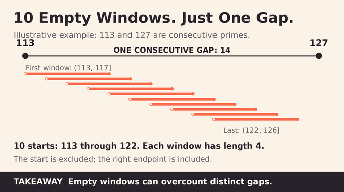
Slide a short window through a prime-free stretch. Many positions describe the same underlying gap. A count of windows weights longer deserts more heavily, whereas a count of prime gaps gives every desert one vote.
The small example below makes the bookkeeping visible. There are no primes strictly between 113 and 127. For length-four half-open windows, starts from 113 through 122 all produce empty intervals.
5.1. Worked Window Count Inside One Prime Gap
| First Empty Window | : contains no prime. |
|---|---|
| Slide One Step | : also contains no prime. |
| Last Empty Window | : is still empty. The next start includes 127. |
| What Was Counted | Ten integer starts, 113 through 122 inclusive. One consecutive-prime gap, from 113 to 127. |
Thus ten empty windows correspond to one consecutive gap. Increasing the underlying gap length creates more empty windows without creating another gap.
A proof based only on plentiful empty windows therefore needs an additional argument. Otherwise, a sparse collection of extremely long gaps could supply much of its interval count. This is the obstacle the adjacent-interval construction is designed to remove. The essential question becomes whether a nearby prime can anchor each successful window with bounded repetition.
6. The New Proof Strategy: Two Adjacent Intervals
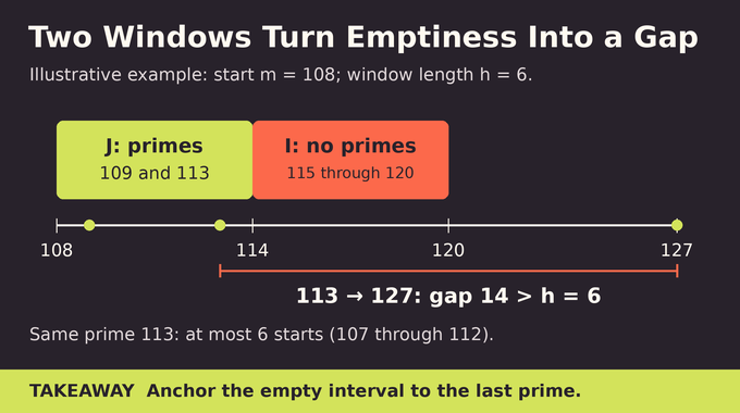
Average over integers . Fix , and choose the integer window length . Consider adjacent intervals:
The target event is a prime in the first interval and none in the second. Select the last prime in the first. There are no primes between it and the end of the second interval, so its successor lies more than away.
The proof does not identify a prime in every first interval. It constructs nonnegative weights under which the first interval retains detectable prime mass while the second becomes nearly prime-free.
For each block of shifts, define as the sum of over its primes. This is a logarithmically weighted count. It is positive exactly when a prime occurs, and every nonzero value is at least one because the primes exceed .
7. Constructing the Nonnegative Sieve Weight
The construction uses smooth divisor sums. Each term sums products of Möbius values over divisors of shifted integers, multiplied by a smooth function of their normalized logarithms. The Möbius function vanishes on numbers with repeated prime factors and alternates sign on squarefree numbers.
Let be the second block’s shifts. For a subset of those shifts, denote this divisor sum by , where is its size. Assemble all dimensions through a finite maximum :
More explicitly, for distinct shifts the building block is:
The divisor variables describe arithmetic constraints, while smoothness makes their correlations analytically tractable. The sum itself is signed. Nonnegativity enters only after the full collection of terms is squared.
The cumulative functions come from smooth, symmetric functions supported where coordinates are positive and their sum is below . Their signs are chosen later. Squaring removes any negative weight:
Here is the limiting average of the square. Proposition 2.1 requires five estimates, with denoting the ordinary average over starting integers.
7.1. The Five Estimates and Their Jobs
| Normalized Mass | . Keeps a nonvanishing total weight. |
|---|---|
| First-Block Prime Mass | . Preserves a prime detector before the empty block. |
| Second-Block Suppression | . Makes unwanted primes inexpensive to discard. |
| Detector Moment | . Prevents prime mass from concentrating on too little weighted mass. |
| Weight Moment | . Converts weighted success into many ordinary integer starts. |
Crucially, is independent of the suppression tolerance . The final weight bound may depend on it. These are separate requirements with separate jobs.
8. The Key Innovation: Cancellation Between Adjacent Dimensions
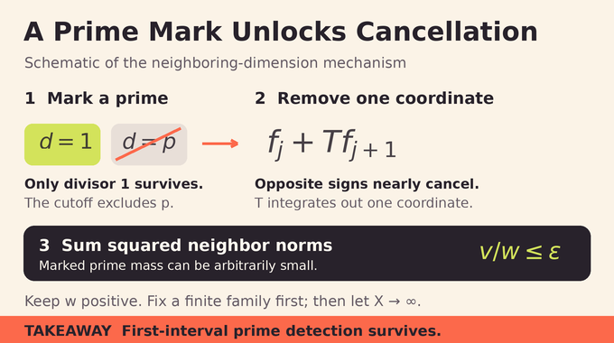
Orthogonality simplifies the unmarked square. When two different shift subsets are paired, an unmatched coordinate forces a mixed derivative onto a coordinate face, where it vanishes. Matching subsets supply the surviving squared norms.
A prime mark inside the second interval changes this pairing. At that prime, the corresponding divisor can only be one in a nonzero term. Its other possible value, the prime itself, violates the support cutoff. Removing this coordinate couples dimensions and .
Define by integrating out the last coordinate. With and , Proposition 3.1 gives the following squared-integral norms:
The construction places alternating product profiles on roughly neighboring levels near . Integration makes adjacent profiles almost match, and their opposite signs nearly cancel. A smooth cutoff preserves the support restriction. The one-dimensional profile has integral of its square equal to one and integral . Rescaling its coordinates by makes integration contribute . Combined with the coefficient ratios, the remaining mismatch is governed by , small for levels near the top. Endpoint costs shrink as the number of selected levels grows, while concentration estimates control cutoff errors.
Consequently approaches one and approaches zero across these auxiliary families. Choose one sufficiently large finite dimension, freeze that family, and only then let tend to infinity.
9. The Analytic Foundation: Moment Bounds and Prime Distribution
Cancellation requires arithmetic estimates, not just formal manipulation. Expanding divisor products imposes congruences on the starting integer. The Chinese remainder theorem combines compatible conditions into residue classes. Incompatible conditions contribute nothing.
With a prime mark, Bombieri–Vinogradov controls prime-distribution errors averaged over the resulting moduli. The support restrictions keep the relevant moduli below its usable range. This does not assume uniform prime counts inside every logarithmic interval. The support budget concerns the sum of normalized divisor coordinates, not the number of coordinates. Thus a large fixed dimension can still fit the required small support. That separation is what allows the cancellation construction to coexist with the available distribution theorem.
Fourier analysis then separates the smooth-function contribution from the singular series, which records local divisibility obstructions. Averaging that series over shifts supplies the constants needed when the subset expansions are summed. The manuscript proves errors uniform in those shifts for each fixed family.
Two moment controls must remain distinct. The bound for detects primes in the first block with a family-independent constant. The bound for later prevents the squared weight from concentrating on too few starts. The detector uses six unmarked divisor factors as majorants, avoiding an asymptotic requiring two prime marks.
Signed arithmetic cancellation also features in our two-point Chowla explainer, but its correlation problem and mechanism differ.
10. From Weighted Intervals to Positive-Density Prime Gaps
First apply weighted Cauchy–Schwarz to the event that the first interval contains a prime:
Its limiting lower bound is . The weighted mass of starts containing a prime in the second block is at most , because its nonzero prime count is at least one. Choose . A positive weighted mass remains on successful adjacent pairs.
Why keep the detector constant independent of the family? Suppression is strengthened by choosing a larger family. If that simultaneously destroyed the lower bound for finding a first-block prime, subtracting unwanted starts might leave nothing. Proposition 3.1 prevents this circular loss.
A second Cauchy–Schwarz application uses bounded to turn this into at least ordinary starts for some fixed .
Now comes the decisive multiplicity bound. Selecting a particular last prime requires . There are at most such integers, regardless of how distant the next prime is. Thus there are at least distinct qualifying gaps, of order .
Choose to make these gaps exceed eventually. Finally set . The selected primes lie below , and the prime number theorem converts the count into a positive multiple of . This proves the bound for every sufficiently large initial segment.
11. How the OpenAI Proof Answers the Erdős–Prachar Question
Erdős and Prachar asked whether the sequence increases on a positive-density set of indices. Cross-multiplication gives the exact equivalence:
The prime number theorem gives . Eventually the ratio on the right is below twice that logarithm. Apply Theorem 1.1 with : its positive-density set of large gaps supplies a positive-density set of ratio increases. Discarding finitely many indices changes no lower density.
OpenAI’s published Lean scope document identifies a formalized supplement for this prime-ratio corollary. It does not describe the entire main theorem as formally verified. We have not independently rebuilt that supplement.
The distinction between a mathematical argument and its formalization scope also guides our Fermat proof-verification explainer. Here, the narrower published scope must accompany any statement about Lean verification.
12. What the Result Establishes and What Remains Open
The OpenAI prime gaps proof establishes an asymptotic lower-frequency guarantee in its manuscript. It does not calculate an exact universal fraction or prove an exponential tail such as . Related Poisson predictions require stronger statements and, in the cited conditional work, additional hypotheses.
Nor does it settle Cramér’s conjecture about maximal gap growth. Bounded-gap theorems concern small distances, while record searches concern extreme individual examples. None is interchangeable with the prime gap distribution question answered here.
For developers, the paper demonstrates no faster prime generator, factoring method, or measured cryptographic improvement. Its reusable conceptual lesson is how to design weights that suppress an event while preserving a neighboring detector and controlling duplicate observations. Our Inverse Goldbach analysis examines a separate sieve-based problem about the structure of primes.
Large prime gaps now have a stronger frequency statement to examine, with precise quantifiers and an identifiable counting mechanism. Follow Binary Verse AI for research explainers that connect the theorem statement to the argument, its verification scope, and the questions it leaves open.
What are large prime gaps?
A large prime gap is the distance between consecutive primes that is unusually large relative to their typical local spacing. The prime number theorem gives an average scale of approximately , so the paper examines gaps exceeding for any fixed positive constant .
Does the OpenAI proof show that unusually large prime gaps occur frequently?
Yes, in the manuscript’s precise asymptotic sense. For every fixed , a positive proportion of consecutive prime gaps exceed in every sufficiently large initial segment. The guaranteed proportion depends on and may be very small.
Why couldn’t previous results establish this frequency?
Earlier results established extraordinarily long gaps or counted many prime-free intervals. Neither alone guarantees a positive proportion of distinct consecutive-prime gaps: one exceptionally long gap can contain many empty intervals. Some earlier results did establish positive prime-start proportions for restricted thresholds. The new theorem covers every fixed positive threshold and controls repeated counting.
How does the OpenAI proof count distinct large prime gaps?
It constructs weighted pairs of adjacent intervals, seeking a prime in the first and none in the second. The last prime in the first interval begins a long gap. At most starting integers can select the same prime, where is the interval length. Moment estimates and two Cauchy–Schwarz applications convert weighted success into positive density.
Does the proof determine the exact probability of a large prime gap?
No. It establishes a positive lower bound , not an exact limiting probability or an distribution. Stronger Poisson-style conclusions in the related conditional research depend on additional prime-tuple hypotheses and should not be attributed to this theorem.
What longstanding mathematical question does the proof resolve?
The manuscript answers an Erdős–Prachar question: whether increases at a positive proportion of indices. Such an increase is equivalent to . The prime number theorem and the main result with give the corollary.
Is the entire OpenAI proof formally verified in Lean?
OpenAI’s published scope document identifies a formalized supplement for the positive-density result concerning increases in . It does not describe that supplement as verification of the entire main theorem. This article has not independently rebuilt the supplement, so its published scope should be distinguished from an independent end-to-end verification.