
Two sets of integers, one addition sign, and every sufficiently large prime: that is the deceptively simple target of the Inverse Goldbach Conjecture. OpenAI’s September 24, 2026 manuscript, The Additive Indecomposability of the Primes, presents a proof that this construction is impossible when each set contains at least two nonnegative integers. Even allowing finitely many mistakes cannot rescue it. The argument combines sieve restrictions, character cancellation, Fourier analysis, and binary-tree comparisons. Its decisive move is to preserve two requirements simultaneously: generate every large prime, and stop generating large composites.
Table of Contents
1. What Is the Inverse Goldbach Conjecture, and How Is It Different From Goldbach?
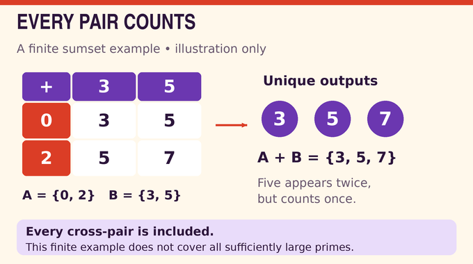
A sumset contains every sum obtained by choosing one element from each input set:
For example, and produce . The repeated representation of five counts once. Crucially, one cannot keep selected pairs and discard the inconvenient sums. Every pair contributes to the same output set. This small example generates only primes, but says nothing about generating the entire prime sequence eventually.
Ostmann’s conjecture, traced to his 1956 treatise, rules out that eventual construction. Classical strong Goldbach instead asks whether every even integer greater than two is a sum of two primes. The outputs and quantifiers differ. This inverse Goldbach conjecture proof does not resolve classical Goldbach.
1.1. Inverse Goldbach Conjecture: Key Facts
| Research Detail | Precise Scope |
|---|---|
| Manuscript | OpenAI, September 24, 2026; included in its October mathematics release. |
| Input Sets | Two subsets of , each with at least two elements. |
| Main Result | Every such sumset differs from the primes at infinitely many integers. |
| Finite Exceptions | Allowed in the conjecture; still insufficient to produce a decomposition. |
| Proof Route | Residue constraints and prime coverage, joined through Fourier and tree comparisons. |
| Verification Scope | Official Lean notes state the full theorem; independent review remains a separate question. |
The requirement is stronger than matching a density or finding infinitely many prime sums. As our Erdős–Turán explainer illustrates, the precise hypothesis on an integer set matters as much as its apparent abundance.
2. What OpenAI Proved: The Exact Statement of Ostmann’s Conjecture
Let denote the positive primes and the nonnegative integers. Theorem 1.1 says that whenever and ,
The symmetric difference, marked by the triangle, contains numbers belonging to exactly one set. Here it records both missed primes and unwanted nonprimes. “Infinite” means mistakes persist arbitrarily far out, rather than disappearing after some threshold.
This also proves that any finite modification of the primes remains additively indecomposable. Removing two awkward primes or adding several composites cannot create a nontrivial decomposition.
One useful consequence sharpens the interpretation: if a candidate sumset contains every sufficiently large prime, it must contain infinitely many composites. Conversely, a sumset producing only finitely many composites must miss infinitely many primes. Individual representations, such as seven being three plus four, remain perfectly possible. The obstruction concerns two fixed sets and all their cross-sums together. Allowing one set to be a singleton would trivialize the question: adding zero to the primes reproduces them. Requiring two elements on each side removes exactly that escape.
3. Why Earlier Sieve Methods Could Not Solve the Inverse Goldbach Problem
Laffer and Mann excluded finite summands. Elsholtz placed hypothetical infinite summands near the square-root scale and excluded three nontrivial summands. Elsholtz and Harper later sharpened the binary counting estimates. These restrictions were substantial, but left room for two sets.
Write , with the same convention for . Earlier upper bounds and the coverage requirement could coexist:
Here allows a fixed multiplicative constant. A lower bound smaller by a logarithm does not contradict the upper bound. Nor does excluding three summands automatically exclude two.
The sharpened Elsholtz–Harper bounds, in their positive-integer convention, range from a constant times to a constant times for each counting function. Even setting both sizes near leaves enough pairs to meet coverage. Size information alone cannot determine how many different prime outputs those pairs produce.
Green and Harper showed that a suitable inverse sieve conjecture would imply Ostmann’s conjecture through a quadratic structural description near the square-root boundary. Large intersections with quadratic images still fall short of that near-containment conclusion. A large structured fragment does not account for almost all of a set. The proof must constrain the remaining elements too, because they can participate in representations of primes that the fragment misses.
The new argument bypasses a general classification. Its “sieve barrier” is this specific insufficiency of earlier restrictions, rather than every limitation of sieve theory. Compare the finite sieve obstruction in the Gaussian moat problem: local restrictions become decisive only after an additional global argument.
4. The First Step: Finite Summands and Complementary Prime Residues
Lemma 2.1 supplies a fixed-shift sieve. If distinct fixed shifts make every sufficiently large prime for , then
The subscript permits dependence on the shifts. If one summand were finite, two of its elements would force the other to have at most a constant times elements. Coverage needs order represented primes. That mismatch excludes a finite summand.
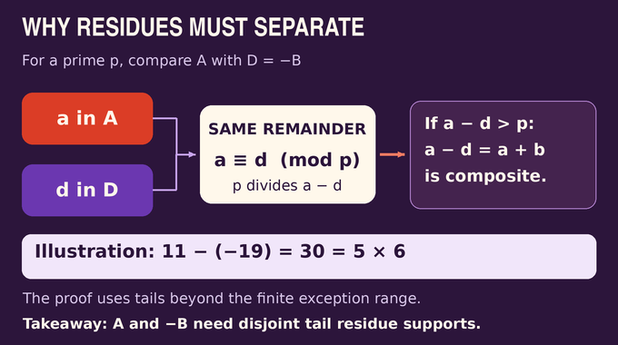
Now assume both sets are infinite and agreement holds above a threshold . Put , so sums become differences. If long-tail elements and share a residue modulo a prime , then is divisible by . Taking both tails beyond , with fixed , makes this difference exceed both and , contradicting primality.
Thus their tail supports are disjoint. Complete them to a partition of the residues modulo . Unoccupied residues can initially go on either side.
5. Collision Stability: Why the Hypothetical Summands Must Be Nearly Balanced
A collision means two independently sampled elements agree modulo a prime. Restricting samples to fewer residue classes raises the probability of collision. Unequal integers cannot collide modulo too many primes, since those primes divide their difference. This is the counting mechanism behind the larger sieve.
Lemma 2.4 gives the bounds used throughout the paper:
Lemma 2.5 refines size control into stability. For diffuse probability measures on opposite long tails, with each point mass at most , it works up to .
Its nonnegative error budget is . The budget combines squared distances from uniform distributions on the respective supports, weighted by , and a density penalty weighted by . Writing , that penalty is , minimized at one half.
Consequently, substantial imbalance or nonuniformity cannot persist across too much weighted prime mass. This is an averaged conclusion, not perfect balance at every prime. The modular collisions in subset sum offer a useful computational comparison for the underlying divisibility count.
6. Quadratic Characters: How the Proof Eliminates Hidden Residue Bias
Balanced supports might still conceal structure. A quadratic character returns one on nonzero squares, minus one on nonsquares, and zero at zero. Translating its input tests whether a support favors squares around a center.
Proposition 3.1 rules out persistent translated quadratic bias on appropriate prime averages, even when every prime chooses its own center. That last freedom matters: assuming one integer center initially would leave an enormous gap.
An amplified even moment turns sustained bias into a large positive weighted sum. Poisson summation rewrites this sum through dual frequencies. Comparing the resulting congruences forces many initially unrelated centers to agree with a common rational number modulo their primes.
The quadratic large sieve then confines positive fractions of both tails to a small family of squarefree kernels, the signed squarefree factors left after removing square factors from the translated integers. Their populations force more collisions than stability permits.
Our Artin primitive-root analysis also discusses quadratic large-sieve estimates. Here their specific job is to eliminate hidden quadratic bias, not classify the summands completely.
7. Beyond Quadratic Characters: Higher-Order Decorrelation
Quadratic tests see only two multiplicative phases. Higher-order characters take other roots of unity and could detect biases those tests miss. Section 4 therefore handles every character order greater than two separately.
Repeated Cauchy–Schwarz transfers create copied prime variables. Smaller and larger anchor variables distinguish their positions, so changing one position exposes an interaction involving the square of a chosen character. That square remains nonprincipal precisely because the original order exceeds two. Quadratic characters required their own argument because their squares are principal.
The anchors also control diagonal contributions, where copied configurations coincide. Ignoring those coincidences would discard terms capable of overwhelming cancellation.
Corollary 4.2 combines the results: outside a set of harmonic prime mass in fixed bands , the normalized transforms have uniformly vanishing correlations against mixed multiplicative characters and additive phases. Harmonic mass means summing , and tends to zero.
As in the two-point Chowla argument, cancellation concerns specified correlations under specified averages. It does not license treating all arithmetic quantities as independent random variables.
8. Fourier Analysis: Why Prime Coverage Forces Nonsparse Additive Transforms
Center the residue indicator and normalize its Fourier transform:
Here is the field of residues and means uniform averaging. The indicator is one inside the support and zero outside. These normalizations give and .
Define , its probability norm. Small , despite unit squared norm, signals concentration on relatively few frequencies. For intuition, a vector with constant absolute value one has both norms equal to one. Concentrating the same squared mass on fewer coordinates reduces its average absolute value. This is a norm comparison, rather than an assumption that every transform has a literal sparse support. Proposition 5.1 supplies an absolute : balanced primes with have harmonic mass at least in , for large .
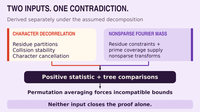
Coverage is essential here. If too much mass had sparse transforms, a nonnegative weight built from those spectra would contract on summand pairs. Its average over primes, combined with coverage, forces an incompatible lower bound.
8.1. Two Inputs That the Proof Keeps Separate
| Proof Input | What It Supplies |
|---|---|
| Composite Exclusion | Complementary modular supports; collision stability then constrains balance and uniformity. |
| Character Arguments | Mixed-character decorrelation, established in Sections 3 and 4. |
| Prime Coverage | A substantial supply of nonsparse transforms, established in Section 5. |
| Combined Use | Positive statistics retain a lower bound while tree comparisons control correlations. |
This proposition does not use character decorrelation. The proof develops the two inputs separately before combining them. Fourier analysis here measures structure, unlike the algorithmic cost studied in our DFT complexity explainer.
9. The Finite-Field Binary-Tree Comparison That Connects the Argument
Transfers generate full binary trees. Leaves carry multiplicative residue variables, while internal nodes reconstruct frequencies and arguments. Comparing two histories means measuring correlations between two such diagrams subject to shared product constraints.
Lemma 6.1 assumes a function vanishes at zero, has probability squared norm at most one, and has small mixed-character correlations. It does not assume a special algebraic formula or a uniform pointwise bound. That flexibility admits the actual residue-mask transforms, which may have large individual values.
For depth , there are leaves. A single diagram has second moment at most . Two diagrams have correlation tending to zero when their paired product constraints have at most components, with fixed.
The proof groups leaves into quartets and finds a cycle in the constraint graph. Reciprocal rescaling around that cycle preserves products. Mellin decomposition, the expansion in multiplicative characters, exposes cancellation while second-moment bounds control the rest. Orthogonality links the character indices around the cycle, so one index is determined by the others. That provides a small correlation factor while bounded total coefficient mass pays for the remaining choices. Preserving this distinction between norm control and pointwise control is essential, as it is in Fourier arguments for Falconer distances.
10. Positive Statistics and Arithmetic Transfers: Preserving the Lower Bound
Section 7 turns the nonsparse supply into tests whose average over a long tail of is positive. Exact tests at smaller primes retain the residue restrictions. Squaring a real averaged test produces a nonnegative smoothed statistic:
Here is a nonnegative smooth weight, the assembled test, and a scale-dependent number of sampled positions. Positivity prevents cancellation from destroying the initial lower bound. Poisson summation converts it into a normalized frequency amplitude.
Further transfers double the history tree while retaining a lower bound. Section 8 justifies replacing arithmetic prime averages by finite-field comparisons. Coprimality and nonzero-frequency conditions stay attached to every history. Repeated internal primes are grouped by equality patterns, not silently declared impossible.
Prime progression estimates retain a possible exceptional real character. The proof handles its conductor through controlled deletions and bounds its surviving contribution where required. These qualifications connect the ideal finite-field argument to actual primes. Without them, the comparison would describe a cleaner model than the arithmetic statistic actually supplies. The spectator primes remain shared across leaves, whereas internal samples are copied according to the transfer rules. Keeping these roles distinct is what makes the eventual local cancellation applicable to the global statistic.
11. The Final Contradiction: Why Primes Cannot Be A + B
Section 9 averages over permutations of the bulk variables. An overlap graph records which leaves share variables between arrangements. Good pairs have few components and tiny correlation. Bad pairs can correlate more strongly, but their fraction has an exponential saving involving .
Fix a sufficiently large transfer depth , put , then let the scale tend to infinity. With a fixed positive constant , the retained amplitude must satisfy both
The second bound is strictly smaller. The order of choices matters: constants and depth are fixed before taking the large-scale limit. Increasing depth during that limit would not justify the uniform estimates being used. This contradiction closes the inverse Goldbach problem.
The official Lean scope notes state coverage of the full theorem, its two-infinite-summands case, and finite modifications of the primes. This article does not report a fresh compilation or independent peer review. OpenAI’s release announcement attributes the results to an internal frontier model.
The Inverse Goldbach Conjecture establishes a structural impossibility, without providing a practical prime-generation algorithm or proving the general inverse-sieve conjecture. Follow Binary Verse AI for source-led explanations and verification updates that keep those distinctions visible.
What is the inverse Goldbach conjecture?
Ostmann’s inverse Goldbach conjecture asks whether the primes, apart from finitely many exceptions, can be expressed as the sumset of two sets, each containing at least two nonnegative integers. It asserts that no such decomposition exists. OpenAI’s September 2026 manuscript presents a proof of this assertion.
Has OpenAI’s proof solved Goldbach’s conjecture?
It proves the inverse Goldbach statement, not the classical strong Goldbach conjecture. The classical problem asks whether every even integer greater than two is a sum of two primes. That assertion is not established by this paper.
What does it mean that prime numbers cannot be written as A + B?
It means no two sets , each with at least two elements, can generate all sufficiently large primes while producing only finitely many composites. Individual primes can still be expressed as sums. The theorem concerns the entire sumset.
Why does the proof allow finitely many exceptions?
The conjecture concerns eventual agreement with the primes, rather than exact equality. The theorem rules out even this more permissive agreement: every nontrivial candidate sumset differs from the prime set at infinitely many integers.
Why did previous sieve methods fail to prove Ostmann’s conjecture?
Earlier methods constrained the possible sizes and residue distributions of hypothetical summands, but those restrictions did not contradict the requirement to cover every sufficiently large prime. The new argument combines residue constraints with additional character, Fourier, and correlation estimates.
How does OpenAI’s proof establish additive indecomposability?
It assumes a decomposition, derives complementary modular supports and decorrelation constraints, then uses prime coverage to supply nonsparse Fourier transforms and build a nonnegative statistic. Binary-tree transfers preserve a lower bound, while comparisons and permutation symmetrization force an incompatible upper bound.
Is the inverse Goldbach conjecture proof formally verified in Lean?
The released official Lean formalization notes state that the formalization covers Ostmann’s full theorem, including the two-infinite-summands case and finite modifications of the prime set. This describes the documented scope. It does not report a fresh compilation by Binary Verse AI, and formalization is distinct from independent peer review.