

Choose the integer 2. Can its powers generate every nonzero residue modulo infinitely many primes? Artin’s primitive root conjecture predicts yes. OpenAI’s October 4, 2026 manuscript Primitive roots for every admissible integer base claims an unconditional proof, covering every integer except −1 and perfect squares. Its quantitative guarantee is a lower bound of order in each sufficiently large interval between and .
That would settle the conjecture’s infinitude assertion after 99 years, but it would not prove the stronger predicted density. Independent verification of the full argument is not established by the materials examined here. For readers following AI mathematical proofs, the substance is a two-part construction: control zeros of specified L-functions, then build primes whose possible obstructions can be removed.
Table of Contents
1. What Is Artin’s Primitive Root Conjecture? The 1927 Problem
Artin’s conjecture on primitive roots fixes an integer and varies the prime . A primitive root generates the entire multiplicative group of nonzero residues: repeated multiplication eventually visits every available nonzero class. Primes dividing are excluded because its residue is then zero.
1.1. Artin’s Primitive Root Conjecture: Key Facts
| Feature | Precise Meaning |
|---|---|
| Manuscript | OpenAI, October 4, 2026; publicly released October 6. |
| Admissible Base | Any fixed integer other than −1 or an integer square. |
| Claimed Count | At least primes in , eventually. |
| Uniformity | The positive constant and threshold may depend on the base. |
| Unresolved Strength | The predicted positive-density asymptotic is not established. |
| Verification | No primitive-root entry found in the current Lean catalogue. |
Infinitude means the supply never ends. Density asks what proportion of primes works, asymptotically. The second statement implies the first, but the reverse need not hold. Similar distinctions between quantitative estimates and infinite-set consequences matter in our Erdős–Turán analysis. The October manuscript explicitly targets the weaker conclusion.
2. Primitive Roots Modulo p: Multiplicative Order and a Worked Example
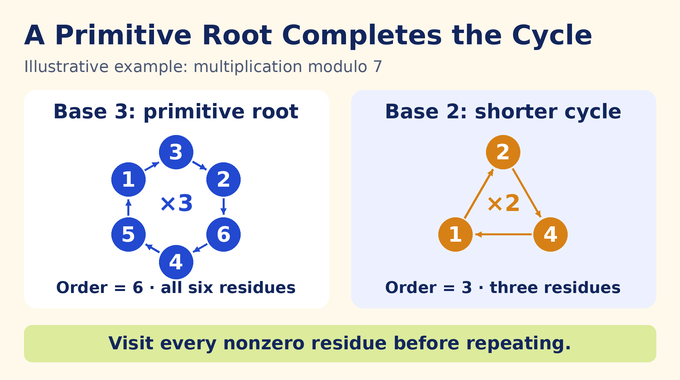
The multiplicative order is the smallest positive integer for which . Fermat’s little theorem ensures that this order divides . A primitive root has the largest possible order:
Modulo 7, the successive powers of 3 give 3, 2, 6, 4, 5 and 1. All six nonzero residues appear. The powers of 2 give 2, 4 and 1, then repeat. Thus 3 has order six, whereas 2 has order three. This is a local calculation, not evidence that either base fails globally.
A shorter test checks each prime divisor of : the residue must differ from 1. For 3 modulo 7, the relevant exponents are three and two. Their residues are six and two. Neither equals one, so no prime factor can be removed from its order. For developers, modular exponentiation makes these checks concrete, although obtaining the prime factors of the group order is a separate computational task.
A computation can certify that a particular prime passes the test. It cannot certify the infinitude assertion by running longer: however many primes a program checks, its list is finite. Conversely, the theorem concerns existence and abundance, without promising an efficient procedure for locating the next suitable prime. These are complementary questions. Keep the integer base fixed when interpreting experimental counts, and distinguish a finite proportion observed in a search window from a limiting density proved over all large scales.
3. Why Artin’s Conjecture Excludes −1 and Perfect Squares
The exclusions express unavoidable algebra. The order of −1 is at most two, so it cannot generate groups of increasing size. A nonzero square modulo an odd prime lies in the subgroup of quadratic residues, whose size is . Its order therefore cannot reach . Zero and one are already excluded as integer squares.
The Legendre symbol records whether is a square modulo an odd prime: it is 1 for a nonzero quadratic residue, −1 for a nonresidue, and zero when . The proof chooses primes where the symbol is −1, eliminating the factor-two obstruction.
Odd perfect powers remain admissible when they satisfy the stated exclusions. For with fixed odd , the constructed primes eventually satisfy . Raising to that exponent then preserves order. Negative squares other than −1 are also included. “Perfect power” and “perfect square” are not interchangeable restrictions.
4. The Previous Barrier: Hooley’s GRH Proof and Heath-Brown’s Result
In 1967, Christopher Hooley’s conditional proof established the predicted asymptotic assuming the Riemann hypothesis for Dedekind zeta functions of the relevant Kummer fields. These fields have the form , with squarefree and denoting the nth roots of unity. This is the specific GRH input behind the historical result.
Unconditional progress left a different quantifier. Heath-Brown’s 1986 theorem implies that at least one of 2, 3 and 5 works infinitely often, and that at most two prime bases fail. It does not identify which member works. Artin asks about every prescribed admissible base.
Likewise, success for almost all bases in a growing range does not settle a fixed base if the exceptional set changes with the range. This is why a population-level theorem cannot simply be substituted for an individual guarantee. Our Goldfeld explainer examines another setting where specifying exactly what is being averaged matters.
5. OpenAI’s Theorem 1.1: The New Quantitative Infinitude Bound
Let count primes with , and . Theorem 1.1 claims that each admissible integer has constants and such that every real satisfies:
Here means the natural logarithm. The interval is dyadic, meaning its endpoints differ by a factor of two. The guarantee concerns every sufficiently large interval of this kind, not merely an infinite subsequence of favorable scales. Since the lower bound grows without limit, infinitude follows.
For base 2, the manuscript claims absolute constants. Across different bases, however, both the constant and starting threshold can change. The theorem statement supplies no practical numerical threshold or generator-search benchmark. As in our irrationality-exponent analysis, an asymptotic conclusion must be read with its actual quantifiers. It does not tell an engineer when a particular implementation becomes useful.
6. Kummer Fields and Complete Splitting: The Central Obstruction
The proof packages failure into the index:
Index one means success. A larger index has a prime divisor , and that divisor witnesses an order shortfall. For primes with , Lemma 2.3 identifies the obstruction through two congruences:
Together they mean that splits completely in . Complete splitting says every residue field above has degree one. In this setting, the roots of the polynomial reduce to distinct elements already in the prime field.
This translation is the central bridge: a modular-exponentiation failure becomes a splitting event countable by analytic number theory. The difficulty is that varies with . Good estimates for one fixed field do not automatically remain good as the possible index divisors grow.
7. Theorem 1.2: OpenAI’s Uniform Hecke L-Function Zero-Free Region
Theorem 1.2 claims that, for every cyclotomic number field containing and every finite-order Hecke character of , the meromorphic continuation of has no zeros in:
A Hecke character is an arithmetic character over a number field, generalizing the role of a Dirichlet character over the rationals. Finite order means its values belong to a finite group. The principal character is included, while its pole at is allowed. A pole is not a zero.
The numerical width is shared across the stated fields and characters, with no conductor or height cutoff. Constants and onsets in intermediate estimates may still depend on the fixed field and character. That distinction is essential: a common boundary does not promise identical numerical estimates everywhere.
This is not GRH, which imposes a much stronger critical-line requirement. The paper develops machinery related to the Quasi-Riemann Hypothesis manuscript, but proves its stated theorem over the specified cyclotomic fields. Section 9 then derives splitting estimates with explicit degree and discriminant control.
The Kummer field itself need not be cyclotomic. Section 9 embeds it into an extension of , applies the theorem through abelian Hecke factorization, and descends the zero exclusion to its Dedekind zeta function. The resulting splitting bound has a main scale and error , uniformly for the permitted growing range of . Both pieces matter. The first decreases with the field degree. The second must remain small even after summing over possible obstructions. A fixed-field estimate alone would not justify that summation.
None of this follows simply from drawing a fixed strip on a diagram. The manuscript also needs bounds for field degree and discriminant, a smooth prime-ideal explicit formula, and a justified passage back to rational primes. Those steps connect analytic uniformity to the eventual count.
8. Cubic Theta Functions, Sextic Reciprocity and the Quadratic Large Sieve
The analytic engine starts with cubic theta coefficients from a selected Kazhdan–Patterson representation. Theta functions organize arithmetic coefficients into objects with transformation laws. Here the coefficients involve Gauss sums, finite sums combining multiplicative characters with additive oscillation.
Sextic twists introduce sixth-root character phases. In a crucial reflected interaction, the local exponents are 1 and −4. Their sum is congruent to 3 modulo 6, turning the interaction into a quadratic character. That conversion matters because quadratic characters can be handled by a quadratic large sieve.
A large sieve bounds the aggregate size of many character sums. It prevents a family of correlations from collectively becoming too large, even when individual sums are awkward. The reflected moment estimate supplies one evaluation of an additive average.
The manuscript’s normalization and Appendix A are substantial proof obligations. They specify the chosen cover, Whittaker factorization and local coefficients. Naming classical theta theory does not verify this specialization. The argument depends on those exact identities carrying through the reflection, including the treatment of unrestricted cube factors.
9. Poisson Summation, Euler Products and Mellin Continuation
The same additive average receives a second evaluation through Poisson summation. This identity exchanges a lattice sum with a sum over dual frequencies. The principal frequency reveals an Euler product, while the other frequencies require separate bounds.
At an eligible prime ideal , the first squarefree theta contribution is , where is its norm and a Mellin variable. Combined with the constant term, this supplies the local factor of a reciprocal Hecke L-function. Remaining terms form a correction claimed to be holomorphic and nonvanishing in the needed region.
The Mellin transform converts scaling into complex-variable analysis. A power saving for the principal inverse-Mellin expression permits continuation across real part one. A zero of the target L-function would create a pole in its reciprocal, contradicting that continuation once cancellation by other factors is excluded.
A conductor large sieve and zero detector control the nonprincipal frequencies. These are necessary safeguards, not optional error bookkeeping: the pole-detection conclusion requires that those frequencies cannot hide the singularity being tested.
10. Constructing Special Primes: Why OpenAI Chooses p = crQ + 1
Analytic estimates become useful only after the proof restricts possible divisors of the index. Proposition 2.1 claims many primes with a controlled predecessor:
Here is prime. Every prime divisor of lies strictly between and . A fixed progression forces quadratic nonresiduosity, with local coprimality requirements ensuring compatibility.
For base 2, the particularly simple choice is , and . Primes congruent to five modulo eight make 2 a quadratic nonresidue. Any remaining prime index divisor must therefore divide .
The geometry of the factor ranges does the work. is so large that an obstruction involving it forces the order to be small. The factors of grow slowly enough to fall within the uniform splitting estimate. Arbitrary primes offer no such tidy division of labor.
11. Marked Type II Estimates and the Sieve That Removes the Obstructions
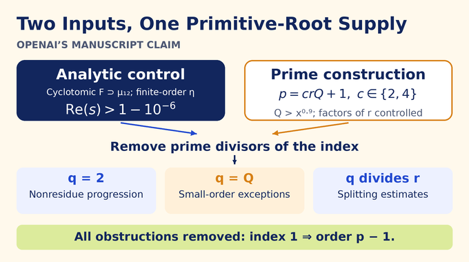
The prime construction begins with weighted integers of the desired predecessor shape, not with a ready-made prime list. Marks require prime factors in prescribed ranges. Type II estimates control bilinear sums involving two varying factors. The paper uses a companion marked-prime theorem and verifies the character and frequency estimates needed for its rough-factor comparison.
Bombieri–Vinogradov distribution supplies averaged information in progressions. A block sieve removes small prime divisors, and Buchstab decomposition sorts surviving composites by their least prime factor. A separate estimate handles composites with two nearly equal prime factors. The claimed comparison leaves a positive prime mass. This is a delicate sieve construction, related in difficulty to the parity obstacles in Chowla’s conjecture.
11.1. How the Remaining Index Divisors Are Removed
| Index Divisor | Removal Mechanism |
|---|---|
| The chosen progression forces the Legendre symbol to be −1. | |
| Order is below ; only candidates are lost. | |
| Uniform complete-splitting estimates yield a total loss . |
Here permits a constant depending on the base. The notation means the ratio to the stated comparison scale tends to zero.
For , an exceptional prime divides some with small . Bounding the logarithm of their product bounds how many primes above can divide it. For , the proof sums the splitting estimate over the permitted range. Both losses are negligible compared with the constructed supply, leaving index one.
12. What OpenAI’s Proof Establishes and Why Artin’s Constant Remains Beyond It
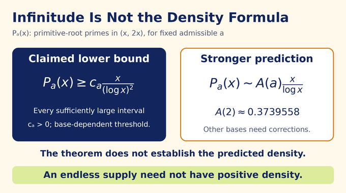
The proposed Artin primitive root conjecture proof therefore combines an analytic exclusion theorem with a carefully sifted prime family. If validated, it establishes infinitude for every admissible fixed base, including 2. The density prediction remains stronger: its natural counting scale is , with a base-dependent constant.
Artin’s constant is approximately 0.3739558, arising from the prime product . It is the predicted density for base 2. Other bases require corrections. Fan and Pollack’s uniform conditional counting theorem explains the base-dependent density framework. The new lower bound neither identifies that density unconditionally nor proves it exists.
As of October 13, 2026, the paper’s directory still identifies the October 4 version. OpenAI’s release announcement describes model-produced results and formalizations of many proofs, not universal checking. The current formalization catalogue contains no primitive-root entry. Our Fermat formalization explainer clarifies why proof discovery and machine checking are distinct achievements.
For Artin’s primitive root conjecture, the next useful evidence is an independently checked argument covering the analytic theorem, the sieve construction and their dependencies. Follow Binary Verse AI’s coverage of AI mathematical discovery for explanations that keep the theorem, its scope and its verification in view.
What does Artin’s primitive root conjecture state?
Artin’s primitive root conjecture states that every integer other than −1 or a perfect square is a primitive root modulo infinitely many primes. A primitive root generates every nonzero residue modulo a prime through its powers. Primes dividing the base are excluded.
Has OpenAI proved Artin’s primitive root conjecture?
OpenAI’s October 4, 2026 manuscript claims an unconditional proof of the infinitude assertion for every admissible base, including 2, with a lower bound of in every sufficiently large dyadic interval. The materials examined as of October 13 do not establish independent verification of the full proof, and the current Lean catalogue contains no primitive-root entry. The stronger density conjecture is not proved by this theorem.
How does OpenAI’s proof overcome the Generalized Riemann Hypothesis barrier?
The proof claims a common zero-free region for finite-order Hecke L-functions over cyclotomic fields containing . Cubic theta coefficients, character sums, Poisson summation and Mellin continuation supply the analytic argument. Combined with specially constructed primes whose predecessors have controlled factors, this replaces the GRH-dependent splitting estimates in the infinitude argument.
Is 3 a primitive root modulo 7, and how can we check?
Yes. The prime divisors of are 2 and 3. The corresponding tests give and , neither equal to 1. Therefore 3 has order six and is a primitive root modulo 7. In contrast, 2 has order three.
Does OpenAI’s proof establish Artin’s constant or the predicted density of primitive-root primes?
No. Artin’s constant, approximately 0.3739558, is the predicted density for base 2, with base-dependent corrections in the general density formula. OpenAI’s claimed theorem supplies a lower bound of order , not the predicted asymptotic of order . It does not establish that density unconditionally.