
At time one, the force stops changing. The computation does not. OpenAI’s September 27, 2026 preprint constructs a viscous fluid whose particle motion can simulate an arbitrarily long Turing-machine run, even after its external force becomes stationary.
For readers searching “Navier Stokes Turing complete,” the precise answer is yes for these specially constructed forced flows. A designated particle enters a designated region exactly when the encoded machine halts. The fluid begins at rest, the geometry and viscosity stay fixed, and the machine determines the force. This is a mathematical universality result, with an exact reachability test. It establishes neither a practical fluid processor nor general regularity for arbitrary fluid data.
Table of Contents
1. Navier Stokes Turing Complete: The Exact Claim
The source is Universal Computation with Eventually Stationary Navier–Stokes Forcing. Theorem 1.1 gives a terminating procedure that converts a deterministic Turing machine and finite input into a smooth external body force. Only that prescription changes between experiments.
| Feature | Theorem 1.1 Guarantee |
|---|---|
| Domain | Fixed flat three-torus , with periodic spatial coordinates. |
| Viscosity | Any fixed positive computable ; the force depends on this parameter. |
| Initial velocity | : the entire fluid starts at rest. |
| Force | Smooth, spatially mean-zero, and stationary for ; all mixed derivatives bounded. |
| Solution | Global smooth solution; unique among classical solutions on every finite interval; uniformly bounded kinetic energy. |
| Observation | Fixed label enters the open strip exactly when the machine halts. |
“Computable” means that an algorithm can approximate the viscosity to any requested rational error. The force likewise has a finite program for evaluating requested derivatives with effective error control. The theorem imposes no efficiency requirement on that program.
Keeping the detector and particle label fixed matters. The compiler cannot move the finish line to wherever a selected execution happens to travel. Its force must produce the prescribed event, with the same observation rule for halting and nonhalting inputs.
2. What the Fluid Equations Actually Describe
The flat three-torus is a unit cube with opposite faces identified. A particle leaving one face reappears through its opposite face. There are no container walls or machine-dependent changes to the metric. The equation is the familiar incompressible Navier–Stokes system:
Here is velocity, is pressure, is viscosity, and is external forcing. The gradient and Laplacian are spatial operators. The advection term describes acceleration as fluid moves through a spatially varying velocity field. Zero divergence expresses incompressibility.
These are Eulerian quantities, measured at fixed locations. The output is Lagrangian: follow one material particle, whose trajectory satisfies , with representing its initial label. The theorem connects a field equation to a particle event. That distinction also separates this paper from the existence-and-smoothness question discussed in our Navier–Stokes Millennium Problem analysis.
The explicit construction chooses zero pressure before any optional projection of the force. This does not remove pressure from the governing equations. It identifies a particular forcing and velocity for which zero pressure satisfies them.
3. What Is New Compared With Earlier Fluid Computation?
Computational universality in fluids predates this manuscript. Cardona, Miranda, Peralta-Salas, and Presas constructed Turing-complete stationary Euler flows on a Riemannian three-sphere. Euler describes inviscid fluid motion. Their construction used an adapted geometry.
Dyhr, González-Prieto, Miranda, and Peralta-Salas subsequently obtained stationary Navier–Stokes universality through cosymplectic geometry, published in PNAS Nexus in 2026. That result uses a suitable metric deformation and the Hodge Laplacian. It already demonstrates that viscosity need not eliminate universal computation in that setting.
The present paper changes the constraints: fixed flat geometry, the componentwise flat Laplacian, positive viscosity, and zero initial velocity. Its programmable ingredient is an external force that eventually becomes stationary. The introduction also acknowledges fixed-metric Euler precedents, including a tape-bounded torus construction. The advance is this particular combination of assumptions, rather than the first discovery that fluid trajectories can represent computation.
4. Why Constructing the Force Is More Than Replaying a Program
Given a smooth divergence-free velocity , one can define a force by subtracting viscosity from its material acceleration:
Substitution then makes an exact solution with . This identity alone would be a weak universality argument if the author first ran a machine, recorded its answers, and replayed them through the force. Such a recipe could never finish compiling a nonhalting execution.
The paper instead compiles the finite instruction table. Every branch becomes part of the geometry. The particle’s current position selects the applicable branch, and the force evaluator never needs to determine which instructions a long execution has visited. This is the substantive meaning of an effective construction here.
A useful analogy is compiling code into a reusable instruction mechanism, rather than storing one execution trace. Finite descriptions can govern infinite behavior. Our Boone–Higman explainer’s discussion of decidability helps distinguish such finite rulebooks from algorithms guaranteed to answer every question about their consequences.
5. Making Machine Instructions Reversible
A Turing machine can overwrite a symbol and lose information. A smooth velocity field’s finite-time flow map is invertible. Two different configurations therefore cannot simply be merged into one configuration by the same fluid motion.
The construction resolves this mismatch by recording history. Its compiled machine has three tape tracks: working data, a temporary head marker, and instruction records. After executing an instruction, it marks the work-head location, scans to the history frontier, appends the instruction tag, advances that frontier, and returns to the marker.
The destination state and written symbol identify the preceding rule. That supplies an inverse on the transition domain. The paper proves this property directly for its seven-row rule schema, following the information-retention principle of reversible computation.
Recording also costs work. One original step requires a finite scan through growing history, so an original machine transition is not automatically one fluid clock cycle. Universality preserves what can be computed. It does not promise equal execution speed or free memory.
For example, overwriting either zero or one with a blank normally hides the previous symbol. An instruction record preserves which case occurred. Particle-map invertibility is compatible with viscosity: it concerns trajectories in a supplied smooth velocity field, not reversing the dissipative PDE for arbitrary velocity data.
6. Encoding an Unbounded Tape in Bounded Coordinates
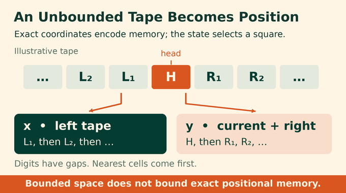
Two planar coordinates encode the tape on either side of the head. Symbols receive distinct odd digits in a base , chosen as , where is the compiled alphabet size. A one-sided tape becomes:
The symbol occupies tape position , and is its assigned digit. Gaps between the allowed digits separate the intervals corresponding to different first symbols. Reading and shifting the tape becomes rescaling or translating these coordinate intervals.
Finite input followed by constant blank tails gives rational initial coordinates. The construction does not require a noncomputable initial oracle. Its idealization appears during execution: arbitrarily deep tape information can occupy arbitrarily fine positional distinctions.
Think of a long positional expansion whose early digits select the next instruction while later digits store memory. A finite-resolution sensor eventually stops distinguishing some of those later digits. Making the mathematical region compact therefore does not impose a finite information capacity on its exact coordinates.
Each control state has its own small square. Initial placement is adjusted so every experiment starts at the same particle label. A halting state is placed in the fixed observation strip. The information fits into bounded space because exact real coordinates have no fixed finite resolution. That is mathematically legitimate and physically demanding.
7. Turning Symbolic Branches Into Incompressible Motion
Each instruction corresponds to an affine map between planar rectangles. A reciprocal scaling, schematically , expands one direction while contracting the other, preserving area. Translations also preserve area. These maps implement tape shifts and state changes.
The challenge is moving whole rectangles smoothly without collisions. Source rectangles are separately disjoint, and target rectangles are separately disjoint. A source may nevertheless overlap a target, so direct simultaneous delivery would be unsafe.
The paper extracts sources in a specified order into parking columns, reshapes them there, and delivers them to their targets in another specified order. Local Hamiltonian pulses provide divergence-free motion while leaving other tracked rectangles fixed.
The resulting period map agrees with each instruction on a neighborhood of its entire source rectangle. Routing bounds also prevent a nonhalting particle from crossing the detector between checkpoints. Checking integer times alone would leave a serious gap in the claimed equivalence.
The paper’s smooth cutoffs equal one around the intended motion and vanish near other parked rectangles. They turn exact affine operations into localized smooth pulses. Effective separation margins justify these choices without first computing the selected execution.
8. How a Stationary Force Keeps the Computation Moving
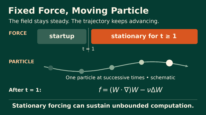
The planar processor ordinarily depends on a repeating phase. A third spatial coordinate supplies that phase, producing an autonomous field . The clock component equals one along the computational corridor, so there. Elsewhere it compensates to keep the spatial mean zero.
A fixed smooth ramp starts the fluid: , with . The ramp is zero near the initial time and equals one from time one onward. The prescribed force becomes:
For , the ramp derivative vanishes and . Everything remaining depends only on position. The velocity is then stationary too, but a particle continues moving through it. A steady river does not require each water parcel to stand still.
Stationary does not mean absent. The force continues compensating for the prescribed acceleration and viscosity. Likewise, spatial mean-zero describes the vector average of the force, not its work on the fluid. Correlations between local force and velocity can still supply energy.
The accumulated computational phase is:
For this ramp, when . Each positive integer compiled phase therefore occurs at physical time . Every finite phase is eventually reached. The force supplies a persistent spatial instruction mechanism, with no time-dependent instruction stream after startup.
9. Why Smoothness Does Not Remove Undecidability
Suppose an algorithm could inspect every force description produced by this compiler and decide whether the designated particle ever enters the detector. Feeding it a compiled machine would decide whether that machine halts. Corollary 6.2 rules this out by reduction to the halting problem.
This does not prevent computing useful finite trajectory segments. It prevents one terminating yes-or-no procedure from correctly classifying the infinite-time event for every instance in the constructed family. A long simulation that has not reached the strip cannot, by elapsed time alone, certify that it never will.
Smoothness, uniqueness, and bounded energy are compatible with this limitation. They control the existence and behavior of trajectories without resolving every proposition about their future. Finite-horizon reliability, such as the question explored in our MAKER analysis of long computations, is a separate requirement from deciding unbounded behavior. The theorem establishes an algorithmic boundary, not ordinary unpredictability from noisy measurements.
10. Finite Precision, Noise, and the Alternative Forces
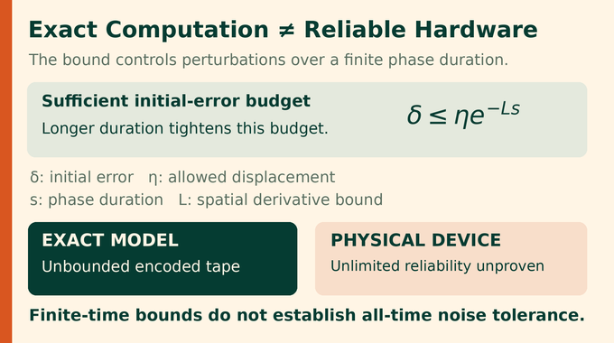
The planar construction provides effective perturbation bounds. If bounds the relevant spatial derivatives, an initial error can grow by at most an exponential factor over a phase interval of length . To keep displacement within , the stated bound permits an initial error satisfying:
This sufficient tolerance depends on the duration. It gives controlled finite-time tubes, not one noise allowance valid for every computation length. The paper supplies no demonstrated physical device, measured throughput, or competitive implementation. Nor does it establish that a fixed mesh can preserve unlimited tape information.
| Construction | Time Behavior | Qualification |
|---|---|---|
| Eventually stationary | Force becomes fixed after time one. | Main theorem; continued forcing is allowed. |
| Periodic | Force has period one from time zero. | Separate construction, still starting from rest. |
| Slow clock | After startup, ; the force tends to zero. | All mixed derivatives have square-integrable temporal spatial-supremum norms; accumulated phase remains unbounded. |
The slow clock accumulates phase logarithmically. It is a different force from the stationary one. Square-integrable force norms are not a proof of finite total physical work. As in our subset sum complexity analysis, an existence theorem and a performance claim require different evidence.
The exponential perturbation estimate is an upper bound, not a demonstration that every trajectory amplifies errors at that rate. It establishes a sufficient finite-time precision budget. It cannot by itself establish either inevitable physical failure or reliable operation for all durations.
11. What the AI Release and Lean Artifacts Verify
OpenAI included this manuscript in its October 6 mathematics release, attributing the collection to an internal frontier model. The release describes Lean formalizations for many results, without claiming that every manuscript is formalized.
The family 376 formalization scope notes, inspected on October 13, describe related sheet programs, decaying-force halting detectors, velocity-field detectors, and box-transport constructions. They do not list this eventually stationary manuscript among the accompanying papers. Formalization of related constructions therefore does not certify every assertion in Theorem 1.1 here.
Readers should distinguish the analytical manuscript, a formally encoded theorem, and independent scrutiny of their correspondence. Our explainers on Fermat’s Last Theorem formalization and checking the scope of a Lean proof develop that distinction. This article analyzes the supplied preprint and documented artifact scope. It does not report an independent Lean rebuild or certify completed peer review.
The fixed-force theorem also contains no finite-time blow-up construction. Clay’s September 11 announcement about the separate Millennium result describes apparent settlement and an unhurried evaluation process. That statement should not be transferred to this computational-universality paper.
12. What Developers and Researchers Should Take Away
The most useful next experiment would isolate a finite instruction family, implement its rectangle routing, and measure how discretization and perturbations affect a chosen computation length. Such an experiment could validate implementation details without establishing the theorem’s infinite-time guarantee. Researchers pursuing hardware would additionally need explicit precision, sensing, and noise budgets.
For AI readers, the contribution is a construction connecting symbolic computation, reversible memory, smooth geometry, and a viscous PDE under tightly specified constraints. It explains how a spatial mechanism can replace a continuing external instruction stream. The distinction between finite description and unbounded execution is the central insight.
The Navier Stokes Turing complete result is compelling on those terms. A fixed force can sustain arbitrary computational duration in an exact mathematical model, while the output question inherits the halting problem’s undecidability. Follow Binary Verse AI’s coverage of mathematical verification workflows for more research explainers that examine what a proof establishes, what its artifacts check, and what practical evidence still needs to show.
What does it mean for Navier–Stokes equations to be Turing complete?
It means that particular solutions can encode the computation of a Turing machine. In this OpenAI construction, a smooth incompressible flow simulates machine transitions through particle motion. A designated particle enters a fixed open region if and only if the encoded machine halts. This is an exact mathematical encoding, not a claim about every Navier–Stokes flow.
How can a fixed force sustain computation indefinitely in Navier–Stokes flow?
The construction supplies a smooth external force that becomes time-independent after . An autonomous three-dimensional velocity field contains a spatial clock and geometric instruction mechanism. The particle continues traversing the encoded computation even after the force stops changing. A nonhalting computation can continue indefinitely, while every finite compiled phase is reached at a finite physical time.
Has OpenAI’s Navier–Stokes Turing completeness proof solved the Millennium Prize problem?
No. This paper establishes universal computation and undecidable particle reachability for specially constructed smooth forced flows. It neither proves regularity for arbitrary initial data nor constructs finite-time blow-up. A separate September 2026 result prompted the Clay Mathematics Institute’s September 11 statement that the Millennium Problem had apparently been settled. Clay described an unhurried evaluation process; that announcement does not validate this different theorem.
Is the Navier–Stokes proof Eulerian or Lagrangian?
It uses both descriptions. The Navier–Stokes equations specify an Eulerian velocity field at fixed spatial coordinates. The computational outcome is Lagrangian: follow a material particle and determine whether its trajectory enters a prescribed open region. The theorem connects the field to that particle event.
Could a real fluid reliably perform the universal computation described in the proof?
The paper does not establish a practically reliable fluid computer. Its construction uses exact positional encoding of potentially unbounded tape information. It provides effective finite-time perturbation bounds for the planar processor, but no fixed precision or noise tolerance is shown to preserve arbitrarily long computations. Physical implementation would require additional sensing, precision, and robustness evidence.