
For 52 years, the Subset sum problem had a stubborn exponential benchmark: split the inputs in half and search at the scale. OpenAI’s October 4, 2026 preprint presents a randomized classical algorithm running in for polynomial-bit inputs in a specified word-RAM model. It promises at least correctness probability for every fixed input, with the time bound holding even on unsuccessful executions. The advance changes worst-case subset sum time complexity, but remains exponential and supplies no practical speedup benchmark.
Table of Contents
1. Subset Sum Problem: What OpenAI Actually Proved
Given positive integers and a nonnegative target , the decision problem asks whether some set of input positions satisfies:
For inputs 3, 7, 11, and 15, target 18 has the solution 7 plus 11. Repeated values remain separate selectable positions. The empty subset is permitted, so target zero is immediately achievable.
1.1. Subset Sum Problem: Key Facts and Scope
| Feature | Precise Scope |
|---|---|
| Manuscript | OpenAI, October 4, 2026 preprint. |
| Main bound | word operations for polynomial-bit inputs, asymptotically. |
| Input | Positive integers, nonnegative target, duplicates and empty subset allowed. |
| Correctness | At least probability for every fixed input. |
| Runtime | Worst-case bound on every execution, including incorrect ones. |
| Model | Uniform classical randomized word-RAM program; preprocessing is charged. |
| Practical evidence | No workload benchmark or competitive implementation established by the manuscript. |
Subset Sum is NP-complete: checking a proposed subset is efficient, while polynomial-time reductions establish NP-hardness. A smaller exponential exponent does not change that classification. The October 4 manuscript is the source of the theorem discussed here.
OpenAI included it in its October 6 mathematics release. As of October 13, the paper’s README still identifies that version, and the published revision history lists no Subset Sum withdrawal. This is a preprint analysis, not evidence of completed peer review or independent reproduction of the full algorithm.
2. The 52-Year Barrier: Why the Half-Exponent Was So Hard to Beat
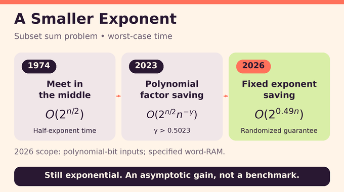
Brute force checks every subset, giving candidates. Horowitz–Sahni’s 1974 meet-in-the-middle subset sum method divides the positions into two halves. Each half contributes about subset sums. Searching for complementary values avoids inspecting every full subset.
Schroeppel–Shamir later preserved that time scale while reducing the space exponent to one quarter. The 2023 algorithm by Chen, Jin, Randolph, and Servedio saved a polynomial factor, with a bound for a constant . That improvement matters, but leaves the exponential rate at one half.
2.1. Algorithm Bounds and What They Measure
| Method | Bound and Qualification |
|---|---|
| Brute force | subsets, with polynomial work per check. |
| Horowitz–Sahni | time in the compared RAM models. |
| Schroeppel–Shamir | Same half-exponent time scale; quarter-exponent space scale. |
| Chen and coauthors, 2023 | , with in their RAM models. |
| OpenAI, 2026 | randomized worst-case word-RAM time for polynomial-bit inputs. |
| Textbook dynamic programming | time for nonnegative target ; pseudopolynomial in the numerical target. |
Dynamic programming tracks achievable totals up to . Its familiar bound is pseudopolynomial because it depends on the target’s value, rather than its binary encoding length. A target written with polynomially many bits can still have exponentially large value. Small-target methods and worst-case bounds in therefore address different regimes.
3. OpenAI’s New Theorem: The Exact Guarantee
Let denote the maximum bit length of any input or the target. For every fixed positive integer , the theorem supplies constants beyond which all inputs satisfying take at most a constant times word operations. The program itself does not depend on .
The machine uses words whose length grows with . Its allowed operations include integer arithmetic, quotient, remainder, bitwise operations, addressing, and random-word generation. Larger arithmetic is charged through multiple operations. Table construction and preprocessing count too. Uniformity means one finite program handles all input sizes without size-dependent advice.
This randomized subset sum algorithm makes no assumption that the integers are randomly distributed. Its probability guarantee concerns internal random choices on each fixed input. Independent repetition and majority voting reduce error, at additional cost.
The answer itself concerns exact equality. Randomness affects whether the procedure answers correctly, rather than permitting a nearby sum. That differs from the controlled numerical approximation studied in our edit distance research analysis.
The ratio between the old and new exponential terms is . That is an asymptotic comparison, not a measured acceleration. The model distinctions resemble those in our integer multiplication explainer: counting operations precisely is essential before translating a theorem into software expectations.
4. The Proof’s Central Insight: Separate Exact Solutions From Modular Aliases
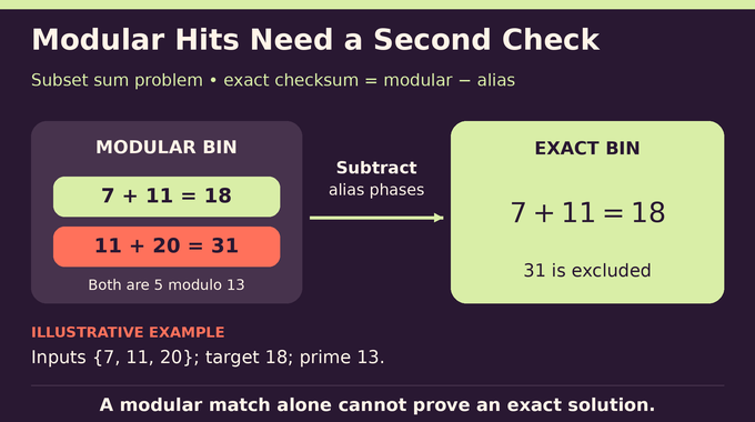
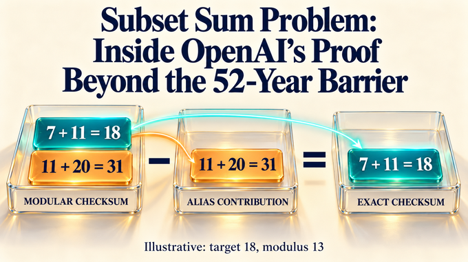
Reducing sums modulo a prime compresses the search space, but merges different integer totals. Call a subset an alias when it reaches the target modulo the prime without reaching it exactly.
Assign every subset a complex phase of magnitude one. Write for the checksum of exact solutions, for the modular checksum, and for the alias set. The organizing identity is:
The algorithm estimates the modular quantity and explicitly removes aliases. Both right-hand contributions can be large even when their difference is zero or a single unit phase. Relative accuracy is insufficient: a small percentage of a huge checksum can overwhelm the signal. The proof must control absolute error.
5. Isolation Lemma: Turning Many Solutions Into One Detectable Target
Many unit phases can cancel. The isolation lemma avoids needing to show that an arbitrary collection of solutions produces a visible checksum.
Choose a power of two between and , and independently draw tie-breaking integers from one through . Transform the weights and targets:
Try all integer offsets from zero through , a quadratic number of targets. Since exceeds the entire tie-weight range, transformed equality forces both original equality and the corresponding tie sum. It cannot turn an original non-solution into a solution.
Among original solutions, a minimum tie-weight subset is unique with probability at least . For each coordinate, fixing the other tie weights leaves at most one troublesome value causing a tie between the best solutions containing and excluding it. A union bound controls failure.
That unique minimum occupies an isolated transformed bin. Its checksum has magnitude exactly one, regardless of phase. Empty bins have checksum zero.
6. Distinct Subset Sums and the Capped Meet-in-the-Middle Test
For a coordinate block , define its support as the distinct transformed sums it can produce. Deficiency measures the savings from discarding duplicates:
Large deficiency means many subsets share totals. The preliminary search builds distinct-sum lists on a random half and its complement, merging translated lists and removing duplicates. Each list has a strict cap near . If both fit, complementary-sum searches return an exact decision. Exceeding a cap produces Continue.
The analysis establishes a dichotomy. If average half-block deficiency exceeds , the preliminary test succeeds with high probability. Otherwise, sufficiently many distinct sums support alias recovery.
Crucially, Continue does not certify the second condition. The proof analyzes the two regimes without conditioning later randomness on that observed outcome. The algorithm never computes the average deficiency.
7. Random Prime Moduli: Where the False Positives Come From
The main prime has approximately bits. It is large enough to limit collisions, but too large to scan all residues within the desired time budget.
For a fixed nonzero discrepancy , only prime divisors of create a false equality. If and a prime is uniformly chosen from the interval starting at and ending before , the paper bounds collision probability by a constant times .
For example, 18 and 31 agree modulo 13, although they differ as integers. A modular hit is a candidate requiring further work. The divisor estimate controls collections of false pairs through averaging, not a claim that every modular hit is exact.
The requirement that discrepancies be nonzero becomes decisive in Section 11. Zero is divisible by every prime.
8. Fourier Checksums: Estimating a Bin Without a Full Fourier Transform
Define , where is the imaginary unit, and draw independent uniform phase residues . A subset’s phase is .
Character orthogonality expresses the modular checksum as a Fourier average:
Here is the target residue and the frequency. Expanding the product selects each input either zero or one time. Averaging over frequencies cancels subsets outside the requested residue bin.
Computing every frequency exceeds the budget. Naive uniform sampling also struggles: at each fixed frequency, the expected squared magnitude over random phases is . The elementary variance bound is too large to obtain sufficiently accurate estimates cheaply.
This proof uses Fourier identities without computing a full transform. It is distinct from the algorithm in our exact DFT complexity analysis, which studies producing the transform itself.
9. Two-Sided Filtering: How OpenAI Finds Useful Fourier Frequencies
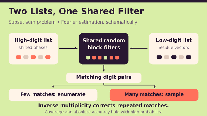
Write a frequency as a high digit times a base plus a low digit. Its phase vector becomes the difference of two vectors, one drawn from each digit list. Random shifts let the algorithm test those vectors separately and find pairs passing the same filter.
The construction uses asymmetric locality-sensitive filtering: the two sides have different scores and acceptance rates. Some coordinates are deliberately ignored. The remaining coordinates receive log-density scores from fixed positive functions on the circle.
An auxiliary, biased shift distribution explains coverage. It favors shifts useful to both sides. Three functions record its expected high score, expected low score, and likelihood-ratio cost. Comparing that distribution with the actual random-table distribution proves that enough trials cover every frequency.
Coordinates are grouped into blocks of roughly square-root size. A pattern records rounded block averages of the three functions, allowing separate thresholds and digit-list lengths for different patterns. There are only subexponentially many patterns, so the algorithm constructs their tables without enumerating all frequencies.
Coverage alone would be insufficient: filters could admit too many entries or inflate variance. Two weighted moment inequalities simultaneously constrain those costs. The new argument balances all three requirements rather than selecting only frequencies with obviously large contributions.
10. Importance Sampling and the Variance Bound
Some patterns have few enough matches to enumerate directly. Others use uniform samples from an implicitly indexed match set. A frequency may appear through several matching tables, so counting every occurrence equally would bias the checksum.
Let be a pattern’s match count and the number of matches representing frequency . For a valid sampled frequency belonging to that pattern, its weighted contribution is:
Other sampled matches contribute zero. Since the selection probability is , inverse multiplicity cancels the overrepresentation. The sample average estimates the pattern’s Fourier contribution without expanding its entire match set.
The filtering constants are explicit, not fitted runtime parameters. Write for the two expected scores and likelihood-ratio cost, and set and . With , , and , the two continuous inequalities are:
Here is the circle and the measure is normalized to total mass one. Appendix A certifies these bounds through 64-point quadrature, rational enclosures, and analytic error estimates. Finite-circle bounds use the slightly relaxed exponent .
These inequalities produce exponentially decreasing mean squared error. The calculation averages under the original phase law, where coordinates at each fixed frequency are independent. It does not incorrectly assume independence after conditioning on filter success.
Subexponentially many patterns and polynomially many targets fit within that error budget. Including arithmetic, the estimator reaches simultaneous absolute error at most . Certified numerical inequalities support this analytic step, rather than constituting a full Lean formalization of the running-time theorem.
11. Recovering Every Alias Without Enumerating Every Subset
Alias extraction uses representations: one subset can be described by many pairs of partial records. A random flip complements chosen selection bits, with signed weights and translated targets preserving a bijection to original subsets.
A shared block occupies roughly coordinates. The remaining coordinates are divided between ordinary left and right sides. Each record includes a subset of its ordinary side and a mask selecting positions in the shared block. Disjoint masks combine into a legitimate subset. Overlapping masks count their common positions twice.
A second, smaller prime and a random residue filter shorten the record lists. Reduced integer sums also require tracking polynomially many possible carries. The low-deficiency regime supplies enough distinct representations that repeated trials recover every alias with high probability.
The essential exclusion comes before checking mask disjointness. Pair enumeration skips every pair whose unreduced signed weights satisfy the exact integer target equation, including overlapping-mask pairs. Sorting makes the forbidden values a contiguous interval, which binary searches skip without visiting.
Every remaining pair has a nonzero integer discrepancy. The random-prime divisor bound can therefore control how many pairs survive. Without that exclusion, exact-equality pairs could dominate the work regardless of prime choice.
Only afterward does the algorithm check disjointness, undo the flip, verify the alias against transformed integer weights, and deduplicate by subset identity. Coverage is probabilistic, but every retained entry is a genuine alias.
12. Assembling the Proof: Correctness, Complexity, and Remaining Limits
Using the same retained phases, subtract the deduplicated aliases from each estimated modular checksum. Combined estimation and arithmetic error is strictly below . Empty exact bins then have estimated magnitude below , while an isolated bin has magnitude above . A threshold of separates them.
Finite arithmetic is part of the proof. Complex phases use rational approximations with polynomially many bits. Record generation, enumeration, and rejection sampling have caps, so unlucky randomness cannot create an unbounded execution. Failure can reduce correctness probability, but never evade the running-time guarantee.
The intermediate operation bound is . For every fixed polynomial-bit regime, the positive gap to eventually absorbs polynomial overhead. Small inputs and inputs outside an exponentially growing bit-length guard use exact meet-in-the-middle fallback.
The OpenAI subset sum proof leaves practical crossover sizes, competitive implementations, and a deterministic equivalent unsettled. It supplies no separate small-space promise. The repository’s formalization catalogue does not list its main result as formalized, so the numerical certificate should not be described as end-to-end machine verification.
There is no quantum oracle or uncharged external computation here. That contrasts with the access assumptions examined in our unitary synthesis explainer.
The Subset sum problem remains NP-complete, and remains exponential. Its significance is the coordinated removal of a worst-case exponent barrier. For developers, keep selecting algorithms by target size, memory, and measured workloads. Follow Binary Verse AI’s research explainers for careful accounts of what algorithmic breakthroughs establish and what still needs testing.
What Is the Subset Sum Problem, and Why Is It NP-Complete?
The Subset Sum Problem asks whether some subset of given integers adds up exactly to a target . A proposed subset can be verified efficiently, and polynomial-time reductions establish NP-hardness. These properties make the decision problem NP-complete. OpenAI’s result improves worst-case exponential running time without changing that classification.
What Is the Time Complexity of the Subset Sum Problem After OpenAI’s Breakthrough?
Classical meet-in-the-middle algorithms established the time scale. A 2023 result saved a polynomial factor. OpenAI’s October 4, 2026 preprint gives randomized time for polynomial-bit inputs in its word-RAM model. Textbook dynamic programming runs in , but the numerical target may be exponentially large in .
How Did OpenAI Break the Barrier?
The proof combines solution isolation, Fourier-based checksum estimation, two-sided filtering, and modular alias recovery. It estimates a modular target bin and removes contributions from subsets matching only modulo a prime. A small absolute-error bound then separates an empty exact bin from one containing an isolated solution.
Is OpenAI’s Subset Sum Algorithm Guaranteed to Return the Correct Answer?
Not on every randomized execution. The theorem guarantees correctness with probability at least for every fixed input, while its asymptotic worst-case time bound for polynomial-bit inputs holds on every execution. Independent repetitions and majority voting can reduce error. Any fixed number of repetitions adds a constant-factor runtime cost.
Does OpenAI’s Result Solve P vs NP or Make Subset Sum Easy in Practice?
No. remains exponential, so this result does not supply a polynomial-time algorithm or resolve P versus NP. The preprint demonstrates no practical superiority on real workloads. Its machine model and hidden constants matter, and no direct cryptographic break follows from the theorem alone.