
The Fast Fourier Transform has spent decades turning quadratic calculations into manageable work. OpenAI now presents a proof that discrete Fourier transform complexity can fall below the familiar scale, at every input length. The improvement is asymptotic, deterministic, and exact, but it belongs to a computational model with unrestricted complex coefficients and supplied roots of unity.
The September 25 preprint gives a logarithmic exponent smaller than one by a minuscule amount. It includes preparation and indexing costs. It provides no practical floating-point speedup. Understanding that distinction makes the result more interesting: the proof challenges a mathematical barrier while leaving everyday FFT engineering largely untouched.
Table of Contents
1. Discrete Fourier Transform Complexity: From Quadratic Work to the FFT Barrier
For a complex input vector , the paper studies the unnormalized DFT:
Here , is the vector length, and selects an output coordinate. The positive exponent follows the manuscript’s convention. Unnormalized means there is no scaling factor in this formula.
At length four, the zeroth output simply adds all four inputs. The other outputs combine them with powers of . Evaluating every output separately takes quadratic arithmetic work. FFT factorizations reuse intermediate combinations to reach work, including arbitrary lengths through convolution reductions.
1.1. Exact DFT Key Facts
| Key Fact | Verified Claim |
|---|---|
| Mathematical Object | Unnormalized, positive-exponent DFT on any complex vector |
| Guarantee | Deterministic and exact at every positive integer length |
| Sharper Bound | , with |
| Simplified Bound | = |
| Arithmetic Model | Unit-cost exact complex arithmetic, unrestricted coefficients, and one specified root |
| Included Work | Scalar preparation, schedule construction, indexing, and array organization |
| Practical Evidence | No useful crossover estimate or demonstrated floating-point speedup |
An upper bound describes an available algorithm. Calling it optimal requires a lower bound for every permitted algorithm. That second statement depends on what operations the model allows.
2. Why Was n log n Believed to Be the FFT Lower Bound?
The FFT’s repeated layers make logarithmic overhead look unavoidable. Historical lower bounds gave that intuition mathematical support, but within specific models.
Morgenstern’s determinant argument concerns the unnormalized Fourier transform when coefficients are bounded. Roughly, each permitted operation can increase the relevant determinant measure only by a controlled amount. Building the Fourier matrix then requires sufficiently many operations.
Ailon’s entropy argument addresses the normalized Fourier transform on coordinates using unitary two-coordinate gates. Such gates preserve the Euclidean norm. Later work also studies restrictions on intermediate conditioning, which measures sensitivity to perturbations.
These restrictions matter. Unrestricted coefficients and exact intermediate values remove constraints used by those arguments. An FFT lower bound for bounded coefficients cannot automatically become a theorem about unrestricted complex-linear computation.
The manuscript also separates its advance from earlier constant-factor improvements. Reducing the leading constant in FFT complexity preserves the growth scale. Reducing the exponent of the logarithm changes that scale. Both are useful mathematics, but they answer different questions about optimality.
3. What OpenAI Actually Claims: The Exact DFT Theorem and Its Assumptions
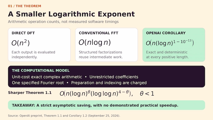
Theorem 1.1 presents one deterministic algorithm for every positive integer length and every complex input. Its sharper running-time estimate is:
The constant is approximately , with exact definitions supplied below. Corollary 1.2 simplifies the estimate to . The iterated logarithm has not disappeared for free. The corollary trades some exponent improvement to absorb it.
Complex field operations have unit cost. Input processing uses addition, subtraction, and multiplication by prepared, input-independent scalars. Division occurs only during preparation, with nonzero denominators established. Complex coefficients and intermediate magnitudes are unrestricted.
Integer addresses use a fixed number of logarithmic-size words. That requirement limits address size, not complex-register precision. One specified root of unity, of polynomial order, is supplied. Other scalars, schedules, and array organization are charged.
The root assumption prevents a hidden algebraic shortcut. Rational field operations alone cannot manufacture roots of arbitrarily large order from rational constants. The algorithm states which root it receives and shows how that root supplies the others. Its access to exact algebraic information is explicit.
OpenAI included the result in its October 6 mathematics release. The relevant achievement is this stated theorem, rather than an inference from the broader AI mathematical proofs coverage.
4. The Two-Coordinate Matrix Behind OpenAI’s New Algorithm
The construction starts with a small complex matrix:
For binary coordinates, its tensor power acts on values. Applying its factors separately costs . The proof seeks a smaller exponent of .
Its starting network has two banks of wires and many auxiliary wires. Each forward invocation performs eight updates: subtract the auxiliaries’ contribution, add the source into the auxiliaries, add their revised contribution, then restore them. Algebraic cancellation produces for arbitrary initial auxiliary values.
Three stages, forward, inverse in the opposite direction, and forward again, exchange the banks with a sign: . Every auxiliary value returns unchanged.
Arbitrary initial values are essential. Recursive calls borrow coordinates already holding data. Requiring fresh zero-filled workspace would break the intended interface and cost accounting. The phase network also appears in the related integer multiplication construction, whose later precision and tape arguments belong to a separate model.
5. How Binary Frames Create a Strict Saving in Tensor Operations
The ingenious step is to replace each scalar wire with an array and attach binary-subspace labels to gates and endpoints. These labels specify coordinate frames , transformations associated with a subspace of a binary vector space.
A scalar gate mixes arrays. A common frame transforms their address coordinates. Those actions commute, allowing adjacent frame changes to cancel throughout the network.
Moving between nested suitable subspaces costs directional kernels for the dimensions added or removed. A directional kernel combines an array with its binary-address translation. On paired addresses it acts like , or its inverse with a translation.
The paper explicitly counts these residual dimensions. If denotes the physical roles and their total directional cost, the saving is . Its exact value is .
This is a finite accounting victory, not an approximate transform. The frames make every physical role contribute correctly, including auxiliary roles. Walsh matrices help establish the identities, but the algorithm does not execute those Walsh transforms. The positive saving will survive padding and become a recursive multiplier.
The binary space organizes addresses, while the stored values remain complex numbers. Confusing those two spaces would incorrectly suggest a finite-field Fourier algorithm. The subspace labels determine which pairs interact. They do not change the arithmetic domain of the input or output.
6. The Recurrence That Breaks the n log n Barrier
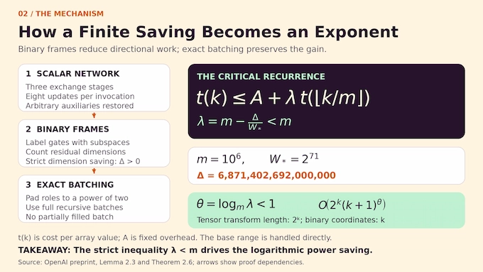
The network uses binary dimensions. Padding its role count to preserves the absolute saving and gives .
Let be the cost of transforming arrays of length , and normalize by their total length: . Splitting into blocks of dimensions yields:
Here is a fixed overhead covering pointwise gates, permutations, leftover dimensions, and batch handling. The recursive argument shrinks by a factor of approximately . Crucially, fiber counts divide exactly into full batches. No partial batch forces wasted workspace or extra transforms.
Unrolling the recurrence gives a geometric sum with about levels. Consequently , where . A single tensor transform therefore costs .
If the multiplier were , this reasoning would retain exponent one. The strict inequality supplies the entire power saving. The algorithm makes that saving survive recursion by transforming arbitrary values on all roles.
The normalized cost isolates overhead per stored value. Recursion reduces the number of active binary coordinates, while batching accounts for all values still being transformed. This distinction explains why a saving in a finite dimension budget can become a bound for an unbounded family of arrays.
7. Newton Interpolation and Toeplitz Matrices: Compiling the Fourier Transform
A faster tensor kernel still needs a bridge to Fourier matrices. Newton interpolation supplies it by viewing as polynomial evaluation at successive powers of a primitive root.
Changing to the Newton basis makes evaluation triangular. Symmetry of the Fourier matrix and uniqueness of triangular factorization then give:
Here is lower triangular, contains its diagonal entries, and is its transpose. Moreover, factors into diagonal matrices and a lower triangular Toeplitz matrix. Toeplitz entries depend on the difference between row and column indices, connecting their action to convolution.
The compiler recursively handles triangular blocks and their cross updates through convolution circuits. It measures the actual register requirements of candidate chunks before choosing a size. Borrowed coordinates can hold arbitrary values and are restored before reuse.
The resulting Fourier word uses exactly coordinates and slots. That is a layer count, not the full arithmetic cost of a length- transform. Preparation is polynomial in . Later, the algorithm chooses small local widths so that preparation remains affordable.
8. Synchronizing Fourier Circuits Without Losing the Complexity Saving
The compiler expresses its words through monomial layers, which permute and scale coordinates, and shear layers, which add a multiple of one coordinate to another. Shears are converted into a fixed pattern using pair slots.
Padding with identity operations lets many local Fourier circuits share a common schedule. Across several axes, a simultaneous pair slot partitions the array into sectors. Choosing a pair on axes produces a sector carrying . Singleton choices leave those axes inactive.
The fast tensor algorithm can now process each sector. However, repeatedly scanning every axis to calculate every entry’s address would reintroduce excessive work.
The paper instead traverses a tree of mixed-radix prefixes. Each extension updates accumulated addresses and coefficients in a fixed number of operations. Because every internal node has at least two children, the total node count is linear in the number of array entries.
This pays for packing sectors, executing them, and undoing the packing. Address arithmetic is part of the proof. Ignoring it could make the advertised saving vanish before any Fourier output appeared.
9. From Special Transform Sizes to Arbitrary Lengths Using Prime Factors
The synchronized construction prefers many small, coprime axes. The working length begins with the product of the first odd primes, taking the largest such product no greater than .
Multiply it by the smallest suitable power of two to obtain with . Thus, the working array remains proportional to the requested input length. The power of two fills a size gap without adding a large difficult axis.
Elementary prime estimates give , while individual factors remain polynomially bounded in . No prime number theorem is needed for this estimate.
Chinese remainder indexing turns the length- Fourier transform into coprime tensor factors, with appropriate permutations. These permutations also use linear traversal work.
The odd-prime axes receive synchronized compiled circuits. The remaining power-of-two axis uses a conventional radix-two FFT. The new algorithm therefore incorporates classical FFT machinery while changing the overall complexity accounting. Merely solving a sparse collection of convenient lengths would not establish the all-length theorem.
10. Bluestein’s Chirp Reduction and the Final Complexity Bound
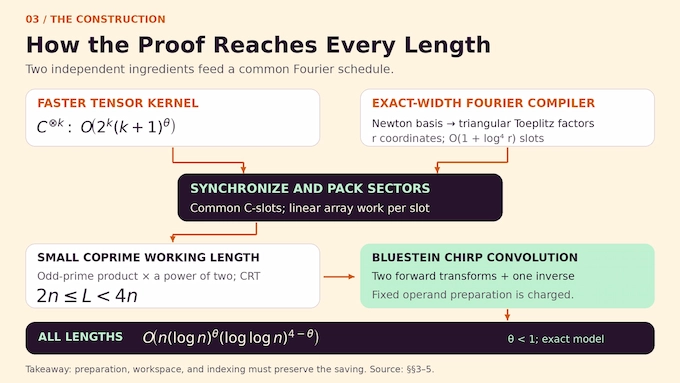
Bluestein’s identity connects the requested transform to convolution. Set . Then:
Multiply input coordinate by its chirp , convolve with the fixed sequence , then multiply output by . Padding at length prevents unwanted wraparound in the required outputs.
The computation uses three full transforms: two forward and one inverse. Transforming the fixed convolution operand counts as preparation. Its pointwise products with variable data are multiplication by prepared scalars, preserving input linearity.
Chirp tables take linear work through successive ratios. A supplied root of order generates the required initial roots, with extraction charged.
Substituting the prime-factor count into the synchronized cost gives Theorem 1.1’s sharper bound. The proof establishes . Eventually, grows more slowly than , producing the simplified corollary. This absorption is asymptotic, not a numerical shortcut for ordinary inputs.
11. Why the New FFT Bound Does Not Translate Into Practical Speedups
The constants are enormous, and the paper offers no useful crossover estimate. Its role padding alone involves arrays in the fixed construction. Exact complex arithmetic treats operations on arbitrarily precise values as unit-cost actions. Hardware does not.
There is also no finite-precision error analysis or numerical-stability guarantee. Unrestricted intermediate magnitudes can matter greatly when arithmetic rounds. The theorem does not establish a faster implementation for existing FFT libraries, GPUs, or signal-processing workloads.
11.1. FFT Time Complexity: What the Bounds Compare
| Method | Operation Bound | Qualification |
|---|---|---|
| Direct DFT | Evaluates every output independently | |
| Conventional FFT | Classical arithmetic upper bound, not universal optimality | |
| OpenAI Theorem 1.1 | All lengths in the stated exact-arithmetic model | |
| OpenAI Corollary 1.2 | Eventually absorbs the iterated logarithm with exponent slack |
Corollary 1.3 extends the same sharper bound to exact linear convolution and multiplication of complex polynomials of degree below . Unlike the input-linear DFT algorithm, it permits general field multiplication for pointwise products of two variable inputs.
It does not establish integer bit complexity, a finite-field result, or a stable numerical algorithm. As with edit distance approximation and practical alignment, the useful question is whether the theorem’s cost model and guarantees match the application.
Polynomial coefficients illustrate the extension directly: multiplying two degree-below- polynomials requires their coefficient convolution, with possible output positions. The proof pads and transforms these coefficients exactly, retaining its arithmetic assumptions throughout.
12. Has OpenAI’s Fourier Transform Proof Been Verified, and What Remains Open?
As checked on October 12, 2026, OpenAI’s Problem 130 formalization documentation reports two scopes. One gives arbitrarily small normalized exact-circuit cost along an unbounded sequence of lengths. A separate uniform formalization gives fixed deterministic programs for every positive length, covering exact DFT and full convolution with the simplified power-saving bound, including root-order selection and scalar preparation.
The supplied-root and unrestricted-coefficient assumptions remain. The synthesis appendix’s extraction, search, and printer uniformization lie outside the selected statements. The documentation does not identify the sharper iterated-logarithm estimate as its uniform comparator statement.
These are repository-reported formalization scopes, without an independent rebuild reported here. The checked primary sources also do not establish completed independent peer review. Formalization and mathematical review answer overlapping but distinct questions, as our Lean proof explainer discusses.
The OpenAI FFT breakthrough changes the unrestricted exact-arithmetic barrier under explicit assumptions. Bounded coefficients, stable numerical computation, and practical crossover behavior remain separate questions. For discrete Fourier transform complexity, a tiny exponent can settle a large qualitative question. Follow Binary Verse AI’s AI and mathematics coverage for explanations that connect new proofs to their actual computational meaning.
What is the time complexity of the discrete Fourier transform after OpenAI’s proof?
Direct DFT computation takes arithmetic operations, while conventional FFT algorithms achieve . OpenAI presents an all-length exact-arithmetic algorithm with running time under supplied-root and unrestricted-coefficient assumptions. The sharper theorem is , where . These are asymptotic operation bounds, not practical floating-point timings.
Why is the Fast Fourier Transform faster than direct DFT computation?
Conventional FFT algorithms reuse intermediate computations through structured factorizations, avoiding the quadratic work of evaluating every DFT output independently. OpenAI’s paper constructs recursive tensor operations with a strict asymptotic saving beyond the familiar scale in its exact-arithmetic model.
Was O(n log n) previously proven to be the optimal FFT complexity?
Not for unrestricted exact complex-linear computations. Earlier lower bounds applied under additional restrictions, including bounded coefficients or unitary operations. OpenAI’s construction permits unrestricted complex coefficients and exact intermediate values, so it does not contradict those restricted-model lower bounds.
How does OpenAI’s algorithm compute the DFT in less than n log n operations?
The proof constructs a finite scalar network whose binary frame changes yield a strict tensor saving, amplifies it through exact recursive batching, and compiles small Fourier transforms using Newton interpolation and Toeplitz matrices. Synchronization, linear-time indexing, coprime factorization, and Bluestein’s chirp identity extend the improvement to every length.
Will OpenAI’s new Fourier transform algorithm make practical FFT computations faster?
The paper demonstrates no practical speedup. It assumes unit-cost exact complex arithmetic, unrestricted coefficients, supplied roots, and enormous constants. It establishes an asymptotic mathematical improvement, with no useful crossover estimate, faster floating-point library implementation, or numerical-stability guarantee.