
Comparing two strings sounds like a small job. Then the strings become long, insertions shift everything sideways, and a simple comparison becomes a search through millions of possible alignments.
OpenAI’s September 24, 2026 manuscript tackles that cost with an edit distance approximation that combines almost-linear expected runtime with accuracy arbitrarily close to exact, provided the accuracy is fixed. Its central theorem concerns arbitrary, explicitly stored strings under unit-cost insertions, deletions, and substitutions.
The result estimates a number. It doesn’t reconstruct an alignment, overturn the hardness of exact computation, or demonstrate faster DNA analysis. Those distinctions determine what the breakthrough means.
The interesting story is how the proof makes speed and accuracy coexist. It builds rough estimates, predicts where a good alignment should travel, and shows that searching those restricted regions can preserve accuracy without quietly rebuilding the quadratic table.
Table of Contents
1. What OpenAI’s Edit Distance Approximation Guarantees
Let and . Theorem 1.1 returns a nonnegative integer estimate satisfying
For every fixed rational , worst-case expected runtime is on a logarithmic-word RAM. The expectation is over internal randomness, with the input held fixed. The manuscript supplies the detailed construction.
Edit Distance Approximation: Key Theorem Results and Guarantees
| Key Fact | What the Theorem Says |
|---|---|
| Accuracy | Between the true distance and (1 + ε) times it on the success event |
| Success probability | At least two-thirds |
| Runtime | N1 + o(1), in worst-case expectation |
| Accuracy parameter | Fixed rational value for the asymptotic bound |
| Input | Explicit integer strings, with polynomially bounded symbol labels |
| Output | Distance estimate, without an edit script |
| Equal strings | Zero on every execution |
For example, if and , success means an integer from 100 through 105. The guarantee is multiplicative, so small distances receive proportionally small error allowances.
Crucially, the successful estimate is one-sided. That lower bound is part of the probability event, not an unconditional promise for every run. Equal strings are handled separately and deterministically.
Fixing accuracy means selecting a value such as five percent and then considering longer inputs. The constants and starting threshold may depend on that choice. The paper explicitly makes no claim of polynomial dependence on inverse accuracy, so asking for more digits can change the computational picture substantially.
2. Why Comparing Two Strings Becomes Expensive
Unit-cost edit distance charges one for inserting, deleting, or substituting a symbol. Transforming ACGT into AGT takes one deletion, so the distance is one.
Wagner–Fischer dynamic programming considers every pair of prefixes. If is their distance, its recurrence is
The boundary values are and . Brackets denote an indicator, zero for matching characters and one otherwise.
Edit Distance Approximation: Alignment Grid Operations and Their Costs
| Step in the Alignment Grid | Edit Operation | Cost |
|---|---|---|
| Advance in the source only | Delete a source symbol | 1 |
| Advance in the target only | Insert a target symbol | 1 |
| Advance in both, symbols differ | Substitute | 1 |
| Advance in both, symbols match | Keep the match | 0 |
For lengths and , filling the table takes time. Two rows suffice for distance-only computation, but reducing memory doesn’t remove the work.
In our example, deleting C changes the relative positions of every later match. This shifting is why counting character mismatches at identical positions cannot replace alignment.
3. The Quadratic Barrier and the Earlier Accuracy Tradeoff
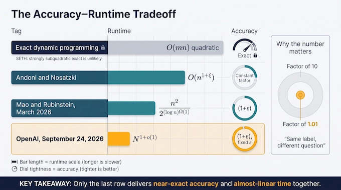
The edit distance SETH lower bound concerns exact answers. Backurs and Indyk showed that a strongly subquadratic exact algorithm would contradict the Strong Exponential Time Hypothesis. SETH is a complexity assumption, not a proved impossibility theorem.
Approximation changes the requirement. Andoni and Nosatzki obtained a constant-factor approximation in time for every fixed . The approximation factor depends on , and the result applies to arbitrary input pairs. It does not offer an arbitrarily small relative error at that runtime.
Mao and Rubinstein’s March 2026 paper reached accuracy in
time for fixed positive accuracy. That is a substantial speedup over quadratic dynamic programming, but it remains a different asymptotic scale from almost linear.
OpenAI edit distance approximation targets the missing combination: near-exact multiplicative accuracy and an exponent tending to one. Its contribution depends on both properties holding together.
This history also explains why “approximate” needs a number attached. A constant factor of ten and a factor of 1.01 answer different questions, despite sharing the same label. Comparing algorithms by runtime alone would erase the central difficulty that this manuscript sets out to address.
Choosing small enough to recover every exact integer answer as input length grows would change the parameter regime. The theorem gives no joint runtime guarantee for that maneuver. It therefore supplies no shortcut around SETH.
4. Coarse Estimates From Shift Trees and Precision Sampling
The algorithm first partitions the source into a hierarchy of intervals. A state pairs one source interval with a candidate target interval. Computing all such substring distances would destroy the runtime budget.
Instead, a shift tree represents possible relative offsets. At an internal node, the schematic recurrence is
Here is the parent shift, a child shift, and the penalty accounts for changing offsets. Leaves compare individual symbols.
Pruning and precision sampling limit how much of this structure gets evaluated. The resulting seed table obeys
simultaneously over every potential interval state, with probability at least 0.99.
“Simultaneously” does real work. Later queries depend on previous answers, so correctness for an isolated, predetermined query would be insufficient.
Each initial entry has a private random stream and is cached after evaluation. Its expected first-request cost remains bounded conditional on the preceding execution. The accuracy event and the work bound are separate arguments, preventing favorable estimates from becoming a hidden assumption about runtime.
5. Connection Penalties Make Local Alignments Compatible
For source interval and target endpoints , define
Only insertions and deletions change length, hence .
Moving target endpoints from to requires at most their total displacement in insertions or deletions. Applying the triangle inequality in both directions gives
Now assign target intervals to consecutive source children. They may leave gaps or overlap. The paper charges the outside endpoint discrepancies and every jump between consecutive target intervals, calling the sum .
Editing the children and repairing those discrepancies yields
For target intervals inside parent , the connection charge is . The overlap is charged too.
Cost cones then combine estimates with endpoint-distance penalties. Their lower envelope makes neighboring values behave smoothly. Wide-action Bellman propagation uses that geometry to build preliminary cost proxies for the next stage.
6. Predicting Narrow Bands Without Knowing the Optimal Path
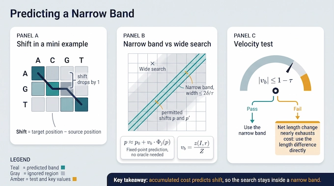
At a source boundary, define shift as target position minus source position. In ACGT versus AGT, it drops after the deletion of C and remains offset afterward.
The algorithm predicts shift using accumulated cost. Let be a preliminary total-cost proxy and set . A prefix ending at shift has proxy cost , so the predicted relation is
This is a fixed-point relation because the prefix cost itself depends on its endpoint. It doesn’t assume access to the unknown optimal alignment.
The velocity test requires . Since is 1-Lipschitz, two permitted shifts with residual tolerance satisfy
and therefore . Substituting the paper’s tolerance gives a narrow band at each cut.
This bounds the band’s width. It does not yet prove that the band contains a sufficiently good action. The comparison-tree argument supplies that missing guarantee.
Some representatives fail the velocity test. When net length change nearly exhausts the predicted cost, the proof can use the length difference to control error directly. It therefore does not force every alignment through the same prediction rule. Geometry determines which case needs the more elaborate band analysis.
7. Cost-Weighted Curvature Pays for Prediction Errors
For analysis, the proof fixes optimal local alignments and rounds their child endpoints. This creates a comparison tree that the algorithm never computes.
Let be preliminary child-cost weights, their shift changes, , and . The curvature quantity is
Expanding the squares proves the identity: the cross terms use , while the final terms use . Zero-weight children have zero shift under the invariants.
The weights measure estimated edit costs, not substring lengths. Curvature therefore measures departure from shift change proportional to cost.
Parent and child weights do not add perfectly. The proof tracks their discrepancies alongside the energy . Summing through the tree cancels internal contributions, leaving controlled terminal, rounding, and propagation charges.
The resulting bound pays for exceptional nodes where prediction fails. At the remaining nodes that pass the velocity test, a coverage lemma places the comparison action inside the computed band. Prediction becomes useful only after this accounting.
8. Entropy-Regularized Choices Control Accumulated Error
Retaining a good action is not enough. The algorithm must select and evaluate actions without adding substantial error at every level.
It uses entropy-regularized prediction over finite mixtures of candidate actions. Entropy spreads probability while the cost terms guide selection. Shared samples support comparisons between nearby rounded representatives.
The relevant online inequality concerns decreasing normalized cost vectors . With , chosen mixtures , and comparator , Lemma 7.2 bounds
Here is the coordinate count and controls regularization. The lemma requires fixed probability mass within child blocks and bounded variation of decrements inside each block. Approximate optimization adds a separately charged error.
The first-crossing argument handles intermediate estimates that drop below true cost. Analysis clips them from below, so underestimation at one node cannot cancel excess elsewhere. This clipping uses true costs in the proof, not an oracle inside the algorithm.
A finite Frank–Wolfe procedure implements the optimization. Exact sampling and rational arithmetic are also accounted for, closing the gap between a mathematical selection rule and executable operations.
9. Repeated Refinement Reaches Accuracy
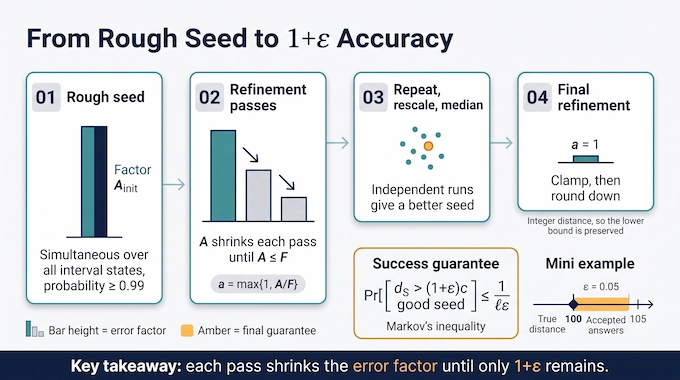
The key refinement theorem starts from a good seed with factor . Setting , it produces
The first bound holds for every refinement outcome conditional on that seed. The second controls positive excess, rather than allowing underestimates to improve an average.
Independent repetitions, rescaling, and medians turn this into a better simultaneous seed. Repeated passes reduce the approximation factor until , making .
For the final refinement, Markov’s inequality gives
Combining this with the probability of seed failure yields the advertised success guarantee. The final value is clamped and rounded down. Because the true distance is an integer, this rounding preserves the lower bound on successful runs.
That sequence is what establishes the 1+epsilon edit distance approximation. Narrow bands alone establish neither the final accuracy nor its probability.
10. Almost-Linear Runtime Requires Its Own Proof
The edit distance approximation time complexity rests on controlling recursive requests. A small error bound says nothing about how many child states an implementation evaluates.
Lazy evaluation computes entries on demand. Caching prevents repeated calculation. Wide searches and optimization reuse previously gathered values, while current-index child requests obey a separate budget.
Along a dependency path, a call either descends the interval tree at the same refinement index or decreases an index or pass. Counting these steps limits the expansion of recursive work. The analysis charges input processing, preprocessing, sampling, data structures, and numerical operations, even when estimates are inaccurate.
The almost linear edit distance bound means the exponent approaches one for fixed accuracy. It does not mean , nor specify a practical implementation.
Likewise, “worst-case expected” averages over randomness for each input. It does not bound every execution by the same runtime. The theorem establishes polynomial workspace on every execution, without a blanket linear-memory promise.
11. The DNA Reality Check
DNA strings fit the mathematical input model. Encoding A, C, G, and T as small integers is straightforward. The scoring and output requirements create the real gap.
Unit-cost edit distance treats every substitution equally and charges each inserted or deleted base separately. Biological alignment can instead distinguish substitutions and use gap-opening and gap-extension penalties. Those objectives require their own analysis.
The output gap matters too. A distance estimate measures similarity but doesn’t identify corresponding bases, mutation positions, or the edit sequence. The theorem supplies no reconstruction guarantee.
Consider a stretch of ten missing bases. Unit-cost scoring charges ten deletions. A model that charges once to open a gap and differently to extend it can favor another alignment entirely. Changing the objective changes which path is optimal, so the present approximation factor cannot simply be transferred to that model.
Then there is the fallback. The manuscript uses exact dynamic programming when or , with defined on the scale of . The large-input branch therefore begins beyond remotely practical input lengths under the stated construction.
That is a decisive qualification for any near linear edit distance algorithm headline. The asymptotic result remains meaningful, but its prescribed thresholds do not establish usable speed on genomic datasets. The OpenAI edit distance proof changes the theoretical tradeoff. Demonstrated biological performance would require further algorithm engineering, an appropriate scoring model, alignment output where needed, and measurements.
This distinction should guide any decision to adopt an implementation.
12. What the Proof Establishes and What to Watch Next
OpenAI’s official Lean scope notes describe the fixed-rational-accuracy guarantee, two-thirds success probability, deterministic zero for equal strings, almost-linear expected work, and polynomial space. They link a comparator statement. This is a formalization scope statement, not a genomics benchmark or proof of practical constants.
The useful next questions are concrete: Can the thresholds shrink? Can the construction become practical? Can its guarantees extend to richer scoring or alignment reconstruction?
For developers evaluating follow-up work, look for stated input sizes, accuracy settings, scoring rules, output requirements, and measured resource use. Those details would connect the existence theorem to an implementation. A runtime exponent alone cannot tell you whether a particular program will finish sooner on the strings you actually have.
Read An Almost-Linear Approximation Scheme for Edit Distance alongside the formalization notes. The breakthrough is the combined accuracy and asymptotic runtime guarantee, with each qualification attached.
Follow Binary Verse AI for research explainers that track those qualifications through to their practical consequences. Edit distance approximation deserves attention because the proof advances what algorithms can guarantee. The DNA reality check tells us what still needs building.
What does OpenAI’s edit distance approximation guarantee?
For every fixed rational accuracy parameter between zero and one, the algorithm returns an integer estimate between the true unit-cost edit distance and one plus the requested relative error times that distance, with probability at least two-thirds. Its worst-case expected runtime is almost linear in the combined string length. Equal strings return zero deterministically.
Did OpenAI solve exact edit distance in almost-linear time?
No. The theorem estimates edit distance within a multiplicative factor of one plus the requested relative error for fixed accuracy. It does not establish an almost-linear algorithm for exact edit distance or provide a runtime guarantee when accuracy becomes increasingly strict as input length grows.
Does the result contradict the edit distance SETH lower bound?
No. The SETH-based lower bound concerns strongly subquadratic exact computation. OpenAI’s theorem concerns approximation with fixed relative accuracy. The two results address different computational requirements.
Does this proof mean DNA sequence alignment is now faster?
No practical DNA speedup is established by the theorem. DNA strings fit the input model, but the algorithm uses unit-cost scoring and returns a distance estimate without reconstructing an alignment. Its stated construction also uses enormous fallback thresholds. Biological scoring schemes and practical genomic performance require further work.
What does almost-linear expected runtime mean?
For fixed accuracy, the runtime exponent approaches one as input length grows. Expected runtime averages over the algorithm’s internal randomness for each input. It does not promise linear time, a particular runtime on practical inputs, or the same time bound on every execution.