
The fraction 355/113 gets astonishingly close to π using just three digits in its denominator. It also points to a question mathematicians have struggled with for decades: how often can fractions achieve that kind of accuracy as their denominators grow?
OpenAI’s manuscript The Irrationality Exponent of π Is 2, dated September 24, 2026, claims an exact answer. It places the irrationality exponent of pi at 2, the value long expected but beyond the reach of previous numerical upper bounds. If the argument holds, it also establishes convergence of the famously troublesome Flint Hills series.
The interesting part is how the paper gets there. It develops an interpolation argument, builds a nonzero determinant, then derives incompatible limits on its size. Supporting Lean materials add a separate layer of evidence, with important distinctions between supplied proofs, selected checking scope, and independent verification.
Table of Contents
1. Pi Was Already Irrational. What Was Still Unknown?
Johann Heinrich Lambert established the irrationality of pi in the eighteenth century, with his proof published in 1768. That means π cannot equal a fraction of integers. A finite decimal such as 3.141592654 is rational, however, because it equals 3,141,592,654 divided by 1,000,000,000.
The new paper addresses the quality of fractions that approach π without ever reaching it.
Irrationality Exponent of Pi: Key Claims and Verification Status
Crucially, the earlier value near 7.1 was an upper bound. Nobody had established that π’s actual exponent was 7.1. The claimed advance closes the gap between a known lower bound and a conjectured exact value.
2. What the Irrationality Exponent of Pi Measures
For an irrational number (x), its irrationality exponent measures which approximation powers occur infinitely often:
[ \mu(x)=\sup\left{\nu>0:0<\left|x-\frac pq\right|<q^{-\nu} \text{ for infinitely many reduced fractions }p/q\right}. ]
Here (p) is an integer and (q\ge2) is a positive integer, with the fraction reduced.
The denominator (q) supplies the scale. A larger exponent demands a smaller error from a fraction of the same denominator size. Numbers with large exponents admit unusually powerful rational approximations repeatedly.
The irrationality measure of pi is another name for this quantity. It measures a particular approximation property, rather than how many decimal digits π has.
Every irrational real number has exponent at least 2. Almost every real number, in the measure-theoretic sense, has exponent exactly 2. That makes 2 a plausible prediction for π, but a statement about almost every number cannot settle one specified constant.
OpenAI claims that for every positive (\varepsilon), there is a threshold (Q(\varepsilon)) such that
[ \left|\pi-\frac pq\right|\ge q^{-2-\varepsilon} \qquad\text{whenever }q\ge Q(\varepsilon). ]
The threshold can change with (\varepsilon). The order matters: choose the extra exponent first, then obtain its eventual bound. The theorem still allows exceptional small denominators and arbitrarily accurate fractions with sufficiently large denominators.
3. Why 22/7 and 355/113 Still Work
Good fractions are compatible with an exponent of 2. The theorem controls a continuing pattern of approximation, so individual successes deserve their applause.
Irrationality Exponent of Pi: Comparing Familiar Approximations
Absolute error measures the distance from π. One exceptionally accurate fraction does not determine the irrationality exponent, which concerns infinitely many approximations as denominators grow.
The continued fractions of pi generate a sequence of especially useful rational approximations, called convergents. Both 22/7 and 355/113 appear in that sequence.
The second is remarkably good because of the continued-fraction coefficient that follows it. A large next coefficient helps explain why the current convergent lands unusually close.
One fraction cannot determine the irrationality exponent of pi. Nor can a finite list of spectacular approximations. The defining condition requires infinitely many successes at a fixed power.
This also corrects a misleading interpretation of “2”: the theorem does not assign every approximation an error of exactly (1/q^2). It describes the boundary between power-law accuracies that can and cannot persist indefinitely.
4. The Previous Barrier Was an Upper Bound
Kurt Mahler’s 1953 work established a finite irrationality exponent for π, including an explicit exponent of 42. That ruled out the extreme rational approximability of Liouville numbers.
Subsequent improvements involved substantial mathematics. Mignotte refined Mahler’s construction. Hata reached approximately 8.016, Salikhov approximately 7.606, and Zeilberger–Zudilin approximately 7.103205334137 in their 2020 publication.
Yufei Bai’s September 2026 preprint claims a further improvement below 7.101862832357 by modifying the Zeilberger–Zudilin integral construction. Its preprint status belongs in any comparison with established published results.
Those bounds constrain what π could do. They leave room for an exponent of 2, 3, or another value below the relevant ceiling.
The OpenAI manuscript proposes a different route to the conjectured endpoint. Its earlier-bound discussion provides historical context, rather than numerical inputs to the proof.
For an irrationality exponent of pi proof, the hard requirement is to exclude infinitely many approximations at every fixed exponent above 2. Shaving another decimal place off an upper bound cannot accomplish that by itself.
5. Assume Too Many Exceptional Fractions Exist
The proof starts with a contradiction hypothesis. Fix an exponent (\nu>2), then suppose arbitrarily large denominators support fractions satisfying
[ \left|\pi-\frac pq\right|\le q^{-\nu}. ]
Because the assumed denominators are unbounded, the argument can select several successively, making each large enough for the requirements already imposed.
This freedom allows their logarithmic sizes to act as separated weights in a multivariable construction. The hypothetical supply of exceptional fractions becomes material for an algebraic object with controlled coefficients.
The order of selection is essential. Requirements chosen after seeing every fraction could create a circular argument. The paper therefore needs interpolation thresholds that can be fixed before the relevant centers are known.
6. Interpolation Produces a Nonzero Determinant
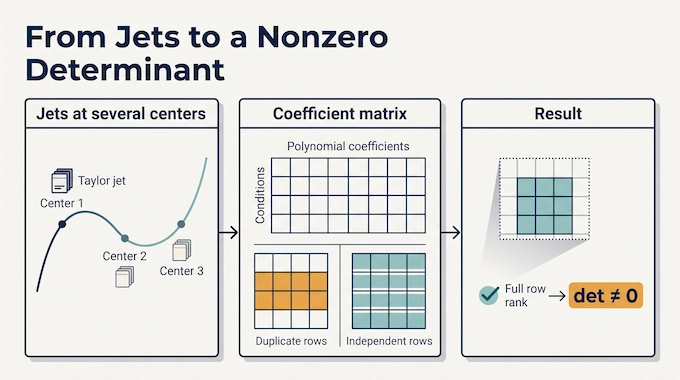
Interpolation usually means constructing a polynomial that matches specified values. Here the requests are richer: prescribe packets of Taylor coefficients at several centers. Such a packet is called a jet.
The paper arranges its variables along logarithmic curves, with additional variables describing movement away from those curves. Different weights control how much polynomial complexity each direction can consume.
A matrix records which polynomial coefficients produce which requested Taylor coefficients. To obtain a useful square determinant, its rows must be independent.
Having more adjustable coefficients than conditions does not guarantee that. Two conditions can secretly ask for the same thing. A spreadsheet with plenty of columns can still contain duplicate rows.
The separated-weight interpolation theorem supplies the missing independence. Its proof uses weighted multiplicities, algebraic curves, logarithmic differentials, and geometric vanishing arguments to establish the required surjectivity.
All polynomial variables share one weighted degree budget. Geometrically, the allowed exponent vectors fill a simplex, a multidimensional version of a triangle. Keeping that full shape matters: the number of interpolation rows and the number of transverse-index groups grow in different dimensions. Increasing the dimension can amplify the cancellation saving relative to the arithmetic costs. The argument needs both this counting advantage and the theorem ensuring that its matrix really has full row rank.
Its crucial uniformity concerns the centers: weights can be chosen before their locations. The final polynomial-degree threshold may depend on the centers. This distinction lets the proof select its exceptional fractions without chasing a moving prerequisite.
7. Arithmetic Limits How Small the Determinant Can Be
Once interpolation provides a nonzero square minor, arithmetic constrains its size.
The matrix involves rational approximations and finite logarithmic expansions. Their coefficients have denominators that the paper explicitly tracks. Scaling rows and columns, then clearing those denominators, turns the determinant into a nonzero Gaussian integer.
A Gaussian integer has the form (a+bi), where (a) and (b) are integers. If it is nonzero, its modulus is at least one. Integer arithmetic provides a floor that small rational errors cannot negotiate away.
Undoing the scaling gives a lower bound for the original determinant. That bound includes costs from denominator clearing and rounding, which the argument must retain.
The purpose is precise: build an object whose arithmetic structure prevents its absolute value from becoming too small. Analysis will now estimate the same object using the supposed exceptional approximations.
8. Analysis Makes the Same Determinant Too Small
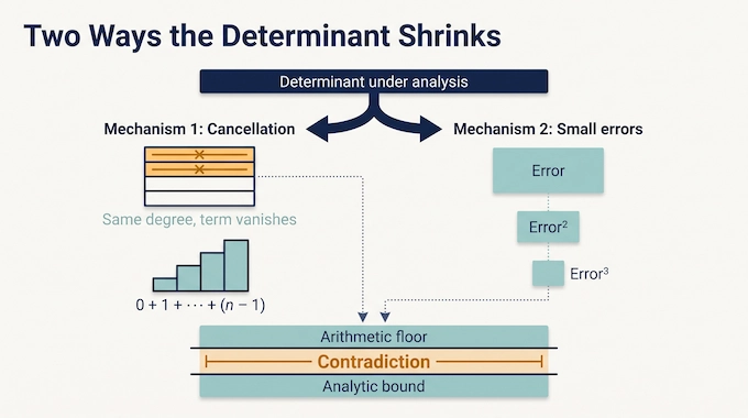
The analytic argument translates the approximate centers toward exact logarithmic periods, (2\pi ij). The identity (e^{2\pi ij}=1) helps organize the resulting entire functions and Taylor expansions.
Two mechanisms supply the decisive savings.
8.1. Repeated Taylor Degrees Force Cancellation
Rows sharing a transverse index test the same family of entire functions. When their Taylor expansions select the same degree, the resulting coefficient rows agree. That determinant term vanishes.
Surviving terms must use distinct degrees within each group. For a group of (n) rows, the smallest possible total degree is (0+1+\cdots+(n-1)), which grows quadratically.
That forced increase in degrees makes the surviving terms smaller. Many rows gathered into relatively few low-weight groups therefore create a strong cancellation saving.
8.2. Higher Indices Supply Small Error Factors
If too few rows occupy those groups, many have large transverse indices. Their expansion coefficients then carry high powers of the tiny rational-approximation errors.
The two cases cover every term. Concentrated low-weight rows pay through cancellation, while high-weight rows pay through approximation errors. The paper bounds both mechanisms before summing the expansion, keeping the arithmetic costs in view.
9. The Contradiction Reaches the Exact Value
The final parameter choices make the analytic upper bound smaller than the arithmetic lower bound. A nonzero determinant cannot satisfy both.
This excludes arbitrarily large denominators meeting the approximation hypothesis for the chosen (\nu>2). Repeating the argument for every such exponent gives the claimed upper bound (\mu(\pi)\le2).
The classical pigeonhole argument supplies the matching lower bound, (\mu(\pi)\ge2). Together they yield the claimed equality.
The paper fixes its dimension, weights, and selected centers before letting the polynomial degree grow. That bookkeeping matters because otherwise quantities described as fixed could silently change during the limiting argument.
The claimed advance in rational approximation of pi therefore comes from a structural contradiction. The result explains a limit on exceptional approximation without supplying a practical algorithm for locating its eventual threshold.
10. Why the Flint Hills Series Would Converge
The classical Flint Hills series is
[ \sum_{n=1}^{\infty}\frac{1}{n^3\sin^2 n}, ]
with angles measured in radians. The (n^3) factor encourages convergence, while occasional tiny sine values create large terms.
The term at (n=355) illustrates the connection. Since (355\approx113\pi), its sine is small. The fraction that makes a lovely π approximation also makes trouble for the series.
Earlier work established that (\mu(\pi)<5/2) is sufficient for convergence. Exponent 2 satisfies that condition comfortably. The equality boundary at (5/2) need not be resolved to obtain this consequence.
The paper also gives a spacing argument. In blocks of comparable denominators, it controls distances to integers and separation between those distances. This bounds the collective contribution of dangerous near-resonances, rather than treating every term as equally dangerous.
That is the heart of Flint Hills series convergence: large spikes must be controlled together with their frequency.
Calculating millions of terms cannot rule out much later spikes. Establishing convergence also does not identify a closed-form sum. The manuscript extends its argument to a generalized family, claiming convergence of (\sum n^{-a}|\sin n|^{-b}) exactly when (a>\max{1,b}).
11. What Has Been Formalized and What Remains Unresolved
The OpenAI pi proof needs several distinct kinds of assessment. The manuscript presents a mathematical argument. Lean materials supply formal proof implementations. Comparator checks are designed to test whether an implementation proves a specified statement using permitted axioms.
As of October 9, 2026, OpenAI’s family-017 scope document describes formalization of the exponent-two assertion, including the eventual approximation inequality and exact supremum characterization. This establishes what the release says its selected formalization covers.
11.1. The Meaning of the Lean Placeholder
A Reddit discussion questioned a sorry in the π comparator file. In this checking arrangement, that file supplies the target theorem, while a separate solution supplies its proof.
The main implementation contains a proof expression for the exponent claim. A placeholder in the target file therefore does not, by itself, demonstrate a missing proof in the solution.
The stronger evidence would be a successful independent check of the complete implementation, statement correspondence, and allowed dependencies. Inspecting a short entry point cannot establish all of that. This explainer reports the supplied materials and their documented scope without claiming an independent rebuild.
There is another important detail. The selected comparator scope excludes the Flint–Hills consequence, but the current main Lean source contains flint_hills_summable. A supplied theorem and inclusion in the selected checking scope are different facts.
11.2. The Stronger Questions Left Open
The irrationality exponent of pi being 2 would still leave meaningful work ahead. The proof gives no effective way to calculate (Q(\varepsilon)), so readers cannot extract a usable denominator cutoff from the theorem.
It also does not establish a uniform positive constant (c) with
[ \left|\pi-\frac pq\right|\ge\frac{c}{q^2} ]
for every fraction. That stronger property is equivalent to bounded continued-fraction partial quotients and is not claimed here.
The result does not establish digit normality, provide a faster π-computation algorithm, or determine the irrationality exponent of every expression involving π. Its scope is substantial and specific.
12. What to Watch Next
The irrationality exponent of pi offers an unusually clear way to understand an AI research claim: a familiar constant, a precise unresolved property, and a proposed argument whose strongest steps can be explained.
If validated, the manuscript would replace a loose numerical ceiling with the expected exact exponent and settle an important convergence problem. The next useful signals are reproducible formal checks, expert assessment of the argument, and precise documentation of any revisions.
For technically curious readers, the lesson is to examine the theorem, the mechanism, and the evidence together. Each answers a different question.
Follow Binary Verse AI at binaryverseai.com for research-paper explainers that unpack what AI claims to have proved, how the argument works, and what verification actually establishes.
1. What does it mean that the irrationality exponent of pi is 2?
It means fractions can approximate π exceptionally well, but cannot repeatedly achieve any fixed power-law exponent above 2 as their denominators grow. More precisely, the claimed theorem gives, for every \(\varepsilon>0\), a threshold beyond which all fractions satisfy \(|\pi-p/q|\ge q^{-2-\varepsilon}\). This is stronger than simply proving π irrational.
2. Why does the accurate fraction 355/113 not contradict the result?
The theorem concerns infinitely many approximations and sufficiently large denominators. It allows individual fractions such as 355/113 to be unusually accurate. One excellent fraction therefore cannot contradict the claimed exponent or establish a different one.
3. Has OpenAI’s proof been independently verified, and what does Lean’s sorry mean?
OpenAI provides formalization materials for the exponent claim. The discussed sorry appears in the comparator’s target statement, which has a separate proof implementation. It does not by itself demonstrate a gap in that implementation. Independent verification requires checking the complete proof, its dependencies, allowed axioms, and correspondence with the mathematical statement.
4. Does the claimed proof settle convergence of the Flint–Hills series?
If the exponent-two theorem is valid, it establishes convergence through the known sufficient condition \(\mu(\pi)<5/2\). The paper also supplies a spacing argument explaining this implication. Convergence establishes that the infinite sum is finite; it does not provide a closed-form value. The selected comparator scope excludes this consequence.
5. Does exponent 2 give practical error bounds or prove that pi’s digits are random?
The paper gives no effective way to calculate its denominator threshold. It also does not establish a fixed positive constant \(c\) satisfying \(|\pi-p/q|\ge c/q^2\) for every fraction. That stronger property concerns bounded continued-fraction coefficients. The exponent result does not establish randomness or normality of π’s digits.