
An algorithm can lose badly even when it may toss coins, adapt its questions, and perform unlimited computation between them. OpenAI’s October 5, 2026 preprint constructs precisely that situation: total Boolean functions where classical randomized algorithms need almost the fourth power of the quantum query count.
The result concerns quantum query complexity, the number of input accesses required to compute an answer. It rules out the conjecture that randomized queries always stay within a cubic power of quantum queries. Combined with an established quartic upper bound, the manuscript identifies four as the optimal universal exponent.
That is the main randomized vs quantum query complexity result. It measures information access, rather than application runtime. The interesting question is how the construction preserves its advantage while requiring a correct answer on every possible input.
Table of Contents
1. What Problem Was Quantum Query Complexity Trying to Solve?
Imagine an input hidden behind individually numbered switches. A classical query reveals one selected bit. A quantum query applies the same bit oracle coherently to a superposition of indices. Interference can reveal structure, but measurement does not hand over every bit simultaneously.
For a function , and denote the minimum worst-case randomized and quantum bit-query counts with error at most one-third on every input. The query cap applies on every execution, including unlucky randomness and measurement outcomes. Computation between queries is unrestricted.
The standard oracle maps to . Here selects an input bit, receives its value through exclusive OR, and represents other workspace. Both competitors access the same input bits, with quantum coherence changing how those accesses combine.
1.1. Quantum Query Complexity: Key Facts
| Component | Meaning And Scope |
|---|---|
| Research object | Specially constructed total Boolean functions, defined on every input bit string. |
| Classical measure | counts bounded-error randomized bit queries, including adaptive strategies. |
| Quantum measure | counts bounded-error coherent bit-oracle queries, with unrestricted computation between accesses. |
| Error guarantee | At most one-third on every input. Query limits hold on every execution. |
| Main conclusion | The universal exponent relating randomized to quantum queries is four. Every smaller exponent fails. |
| Practical scope | No application-runtime benchmark, optimized hardware resource estimate, or measured quantum-device speedup is established. |
A total function assigns an answer to every bit string. A partial function imposes a promise and requires correctness only inside its domain. Promises can support exponential quantum advantages. Totality forces polynomial relationships, leaving the largest possible power unresolved. This distinction also matters when interpreting broader claims about quantum computing and artificial intelligence.
2. Why the Cubic Conjecture Was the Previous Barrier
Grover search gives the familiar quadratic separation: deciding whether any input bit is one takes a linear number of randomized queries but only a square-root number quantumly.
Later constructions moved beyond that benchmark. Aaronson, Ben-David, and Kothari’s cheat-sheet framework achieved a power-5/2 separation, ignoring logarithmic factors. Tal reached . Bansal and Sinha, and independently Sherstov, Storozhenko, and Wu, reached . Certificates hidden at addresses determined by hard partial problems helped drive this progression.
Meanwhile, Aaronson and colleagues established the quartic deterministic upper bound, , where counts exact deterministic queries. Randomized algorithms can simulate deterministic ones, so the same upper bound applies to .
The proposed cubic bound in quantum query complexity asked whether randomness always improved that ceiling to . Nearly cubic examples were consistent with it. The new construction crosses that boundary.
3. What the OpenAI Proof Actually Establishes
Theorem 1.1 of the nearly quartic separation manuscript states that . This parameter is the infimum of exponents allowing a universal constant with for all total Boolean functions. The added one includes constant functions.
For each fixed integer , and sufficiently large powers of four , the paper constructs satisfying:
The positive constants may depend on , which stays fixed while grows. Logs are base two. Their factors prevent reading these statements as exact power laws, yet cannot offset a positive polynomial exponent asymptotically.
OpenAI included the work in its October mathematics release. The checked public formalization catalogue does not list this manuscript as of October 20, 2026. This article treats it as a preprint result, without claiming an end-to-end Lean verification. Our explanation of Lean proof checking covers that separate evidential step.
4. How k-Fold Forrelation Makes the Quantum Advantage Possible
Forrelation detects relationships between sign vectors through a Fourier-like transform. Let be the normalized Walsh–Hadamard matrix, , and the diagonal matrix containing a sign vector . Encoding a bit as , define:
Set . The partial function returns one when , zero when , and is undefined otherwise.
A quantum routine prepares , applies the displayed unitary product in reverse written order, and projects back onto . Success probability is . Each diagonal sign operation costs one phase query. The promise separates two probability ranges, so repetition estimates the answer with a query count independent of for fixed and fixed error.
By contrast, Bansal and Sinha’s Forrelation lower bound supplies classical hardness approaching , up to logarithms. These Hadamard transforms differ from the complex DFT studied in our Fourier transform complexity explainer.
Crucially, an exact Boolean circuit also checks promise membership and computes the answer. Integer Walsh–Hadamard arithmetic gives a fan-in-two circuit of size . A stored evaluation transcript will let the total construction verify those claims locally.
5. How the Proof Converts a Partial Problem Into a Total Boolean Function
There are columns. Each contains an -bit string , plus independent address instances , each holding bits. Independence matters in the later hard distribution. The total function itself imposes no promise or distribution on these strings.
When all address instances are defined, their answers form the address . Column has a certificate cell for every -bit address . Each cell stores circuit transcripts and pointers into all other columns.
A column wins only if its own string is entirely ones, its address answers are defined, and the correctly addressed cell contains valid transcripts and points to a zero in every competing string.
The function outputs one exactly when a winner exists. Malformed transcripts, undefined address instances, and unsuitable pointers simply prevent a column from winning. If no column qualifies, the output is zero. Every input therefore receives an answer.
The enormous cell arrays are deliberate mathematical infrastructure. They create many possible certificate locations, rather than a compact data structure intended for production deployment. The parameter is the number of columns and their string length, not the total number of input bits. Confusing those quantities would give the wrong input-size interpretation.
5.1. The Addressed Certificate Construction
| Component | Meaning And Scope |
|---|---|
| String | Must contain only ones for the column to win. Every opponent must contain a zero witnessed by a pointer. |
| Instances | Their promised Forrelation answers specify the correct certificate address. Undefined answers prevent that column from winning. |
| Cell | Stores a potential certificate at address . Only the true-address cell can certify a winner. |
| Circuit transcripts | Supply proposed gate values. Local checks tie them to actual input bits and certify promise membership and address answers. |
| Outward pointers | Identify one zero in each other column. They establish uniqueness and make genuine-winner comparisons robust to invalid opponents. |
6. Why Outward Pointers Make the Winning Column Unique
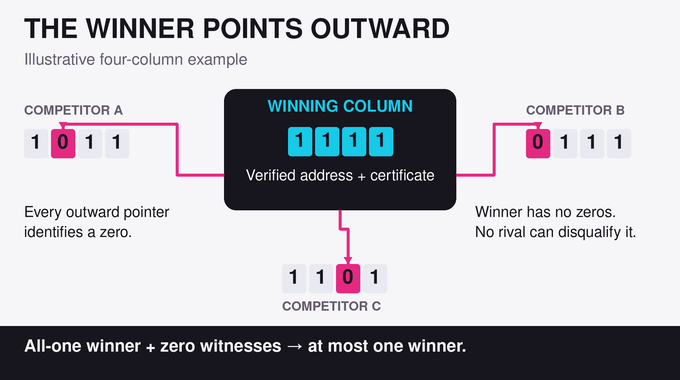
Suppose column three wins. Its string contains no zero, while its certificate identifies a zero in every other column. None of those columns can also have the all-one string required to win. Uniqueness follows immediately.
Pointer direction does more than enforce uniqueness. The winner carries evidence against each opponent. An opponent cannot return the favour because every pointer into the winner lands on a one.
Now let an opponent’s Forrelation input violate its promise. Quantum decoding may produce an arbitrary address and read arbitrary pointers there. It still cannot manufacture a zero inside the winner’s all-one string. The winner’s advantage survives that unreliable decoding.
This asymmetry lets the algorithm compare columns before fully verifying them. Demanding trustworthy comparisons between every pair would discard the freedom that makes totality manageable.
7. How the Quantum Tournament Finds the Winner Despite Unreliable Comparisons
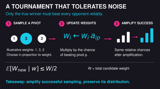
The comparison routine decodes both addresses coherently, retains its workspace, and tests their pointers toward each other. If exactly one finds a zero, that column wins. Otherwise a fixed index rule breaks the tie.
Let be the probability that defeats . A consistent circuit ensures for distinct columns, with . The genuine winner beats every opponent with probability at least . Other comparisons may behave arbitrarily, even without transitivity. A comparison probability can lie arbitrarily close to one-half, so repetition cannot cheaply turn all pairs into reliable fixed outcomes. The proof works directly with their actual probabilities.
The ideal tournament starts with weights . It samples pivot proportionally to its weight, records it, and updates . Writing , complementarity gives, for :
Thus expected total weight falls by at least half each round. Zero weight stays zero. Before being selected, the winner retains weight at least , exceeding one-half for the paper’s choices and . After logarithmically many rounds, omitting it becomes unlikely.
The quantum implementation compares a uniformly superposed candidate against every earlier pivot in fresh workspaces. Conditional success weights multiply, producing exactly the desired sampling distribution. Amplitude amplification raises sampling success while preserving that conditional distribution. The resulting list has at most candidates and costs times polylogarithmic factors in queries. The algorithm never computes the weights numerically. They describe the distribution generated by its coherent comparisons.
8. How Quantum Search Verifies the Winning Certificate
Candidate selection does not certify correctness. For each listed column, the algorithm decodes its address afresh and checks a fixed collection of local conditions.
There is a test for each bit of its own string, each outward pointer, every circuit gate, and the circuits’ promise and answer outputs. Their total number is . Each test costs at most bit queries. A gate test reads its claimed value and at most two predecessor values.
Induction through the circuit ensures that passing every gate test certifies the actual evaluation, rather than merely mutually agreeable invented values. Output checks then certify the address and promise membership.
Quantum search looks for a failed test in approximately tests, with amplification overhead. A real certificate has no failed test to discover. Every false candidate has one at every address. Bounding missed failures and decoding errors gives the required overall error below one-third and the stated quantum upper bound.
Here amplification supports bounded-error verification. The probability-one objective in exact quantum factoring is a different correctness requirement.
9. Why Randomized Algorithms Cannot Easily Discover the Planted Winner
The classical proof couples two input distributions. First, place one independently uniform hidden zero in every string , draw all address instances independently from a hard promised distribution, and leave certificate cells blank. This is a zero-input because no column is all ones.
Next choose a uniformly random column . Erase its zero and fill its true-address cell with correct transcripts and pointers to every other hidden zero. This creates a winner and therefore a one-input.
The inputs differ only at the erased zero and inside that filled cell. Until an algorithm queries one of those locations, both executions receive identical answers and choose identical subsequent queries.
Classical hardness therefore becomes an information-access argument: either discover the removed zero in the randomly selected column, or reach its hidden certificate. For queries, the first event has probability at most . The remaining task is to bound adaptive certificate hunting.
10. How the Adaptive Direct-Product Argument Proves Classical Hardness
Set . For sufficiently large , this is below . Yao’s minimax principle supplies a promised-input distribution where every deterministic depth- strategy succeeds with probability at most two-thirds.
For independent instances, the capped direct-product lemma bounds the probability of guessing every answer by , even when queries interleave adaptively. The cap applies separately to each instance. Conditional on a complete transcript, the independent inputs retain separate conditional laws. Multiplying their best remaining success probabilities gives a supermartingale, whose expectation cannot increase.
Call a column heavy if it receives more than address-instance queries in total. At most columns qualify. A uniformly planted winner is heavy with probability at most . For nonheavy columns, a simulator stops before exceeding the cap. Applying direct product to that simulation avoids wrongly assuming that conditioning on nonheaviness preserves independence.
Union-bounding all possible certificate queries gives total distinguishing advantage at most:
Choosing makes this less than one-third for large , contradicting the gap required by a correct bounded-error algorithm. This is a classical lower bound paired with a quantum upper bound, rather than a new quantum query complexity lower bound.
11. Why the Nearly Quartic Separation Finally Disproves the Cubic Conjecture
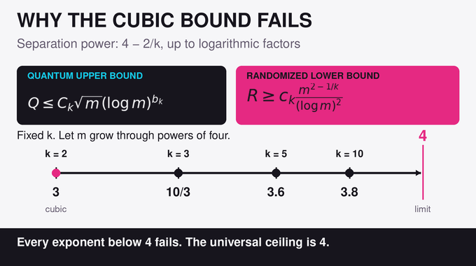
Ignoring logarithmic factors, the bounds compare classical queries with quantum queries, giving the power . For , that is , already above cubic. Larger fixed approaches four.
For any proposed universal exponent , choose fixed so . The ratio of the classical lower bound to then diverges because its positive power of outruns every fixed logarithmic factor.
The existing ceiling completes the argument. Block sensitivity counts disjoint groups of bits whose flips change an answer. The adversary method bounds it by . Huang’s signed-cube method, combined with the adversary bound, also gives exact polynomial degree . The deterministic inequality yields the quartic ceiling.
The OpenAI quantum query complexity proof therefore identifies the optimal exponent, not an exact fourth-power equality for one fixed family. Developers still need gate counts, memory costs, and implementation evidence. Our quantum circuit resource analysis explains why those measurements matter.
For researchers, the reusable ideas are robust probabilistic comparisons and adaptive address hardness. For AI readers, the evidential standard is equally useful: inspect the theorem and its verification scope before treating a model-generated manuscript as settled knowledge. Follow Binary Verse AI for quantum query complexity explainers that trace claims through their assumptions, proof mechanisms, and practical limits.
What is quantum query complexity?
Quantum query complexity measures the minimum number of oracle queries a quantum algorithm needs to compute a function with a specified error probability. In this paper, counts worst-case bit queries with error at most one-third on every input. Computation between queries is unrestricted, so it does not measure total execution time.
What does the OpenAI quantum query complexity proof establish?
The preprint establishes that the optimal universal exponent relating randomized and quantum query complexity for total Boolean functions is four. Its construction achieves separations approaching a fourth-power relationship, ruling out every smaller universal exponent, including the conjectured cubic bound.
Why was the cubic quantum query complexity conjecture disproved?
The conjecture proposed that every total Boolean function satisfies . The manuscript constructs families for which the ratio grows without bound. No universal cubic upper bound can therefore cover all total Boolean functions.
Why does the proof use total Boolean functions instead of partial functions?
Partial functions impose promises that exclude some inputs and can permit exponential quantum query separations. The challenge here was to establish the strongest universal exponent for functions defined on every input. The construction embeds hard Forrelation instances in a total function whose candidate certificates can be tested even when address instances violate their promises.
What role does Forrelation play in the nearly quartic separation?
The proof uses k-fold Forrelation to generate answers that quantum algorithms can obtain with few queries on promised inputs but randomized algorithms find expensive to determine. Multiple independent answers form hidden certificate addresses. Exact circuit transcripts certify those answers, while outward pointers and a probabilistic tournament allow the quantum algorithm to locate and verify a winner efficiently.
Why is the separation called nearly quartic rather than exactly quartic?
For each fixed integer , the bounds yield separation powers approaching , up to logarithmic factors. Increasing the fixed parameter makes this power arbitrarily close to four, ruling out every smaller universal exponent. The paper does not establish an exact fourth-power equality for one fixed family.
Does this proof mean quantum computers are four times faster than classical computers?
No. Four is an exponent in an asymptotic oracle-query relationship, not a fourfold practical speedup. The result concerns specially constructed Boolean functions. Quantum gate costs, data-access implementation, memory requirements, and hardware performance are outside this query-count comparison.