
A fractal can contain infinitely many points and still occupy no area. Can its pairwise distances nevertheless occupy a positive length on a ruler? The Falconer Distance Conjecture predicts exactly when that must happen. OpenAI’s September 23, 2026 manuscript presents a proof in every integer dimension : a compact set whose Hausdorff dimension exceeds determines a distance set of positive Lebesgue measure, without additional regularity assumptions.
The claimed advance reaches the conjectured sharp threshold. Its machinery combines directional geometry, Fourier estimates, and a multiscale accounting argument. Understanding the result requires separating its precise mathematical conclusion from stronger statements about fixed observation points, endpoint sets, or practical algorithms.
Table of Contents
1. Falconer Distance Conjecture: The Result at a Glance
Theorem 1.1 of the all-dimensional research manuscript gives a qualitative existence result. “All dimensions” means every finite integer dimension from two upward. It does not mean fractional ambient spaces or arbitrary notions of distance.
| Feature | Precise Scope |
|---|---|
| Ambient space | Euclidean space , for every integer . |
| Input set | Compact with Hausdorff dimension strictly greater than . |
| Conclusion | Its Euclidean distance set has positive one-dimensional Lebesgue measure. |
| Additional structure | No Ahlfors regularity, product structure, prescribed Fourier decay, or equality of Hausdorff and packing dimensions. |
| Excluded conclusions | No assertion at equality and no sharp-threshold pinned-distance theorem. |
| Evidence | A 64-page manuscript and a repository-described Lean formalization of the main theorem. |
The paper supplies the analytical argument. OpenAI’s repository identifies the formalization’s scope. Those are different evidence layers, and neither should be casually relabeled as independent community acceptance. This article explains the submitted result rather than claiming to reproduce its full verification.
2. What the Distance Set Formula Actually Measures
For a compact set in Euclidean space, collect the ordinary lengths between every pair of its points:
This is the Falconer distance set. Its elements are nonnegative real numbers, regardless of how many coordinates the original points have. A finite triangle produces only finitely many distances. Falconer’s question concerns infinite sets whose geometry persists through arbitrarily fine scales.
Hausdorff dimension measures that fine-scale size using covers by small sets. A value such as 1.2 describes a set more substantial than a one-dimensional object in this covering sense, while still potentially occupying zero planar area. The statement is:
Here denotes Hausdorff dimension, and the quantity on the right is ordinary length measure. Positive length is stronger than Hausdorff dimension one. A set can have dimension one yet zero length, a distinction also central to Kakeya’s dimension-versus-volume problem. Positive length also does not, by itself, promise an interval.
For a concrete reading, imagine a compact planar fractal with Hausdorff dimension 1.2. The stated theorem guarantees positive length for its distance set even if the fractal itself has zero area. A compact three-dimensional set of dimension 1.2 does not meet the hypothesis, because the threshold there is 1.5. The comparison concerns dimension relative to the surrounding space, not merely whether a set looks intricate in a picture.
3. Why Half the Ambient Dimension Is Sharp
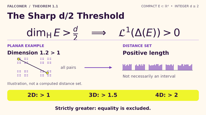
In the plane, the hypothesis becomes dimension greater than one. In three dimensions, it becomes greater than 1.5. In four dimensions, greater than two. These are strict inequalities, however close a particular set lies to the dividing line.
Falconer’s lattice-based constructions explain why the dividing line cannot simply be lowered. They arrange many points while forcing extensive repetition among pairwise distances. Suitable limiting constructions reach the critical dimension while leaving the distance set with zero length. Thus large point populations alone do not prevent distance concentration.
The new argument must exploit the extra dimensional room above the threshold, even when that room is arbitrarily small. It makes no universal positive-measure claim at equality. “Sharp” describes the dividing threshold, not an endpoint theorem.
The lattice intuition also explains why counting points is insufficient. Different pairs can realize the same length, so the number of pairs can greatly exceed the number of distinct distances. Passing from finite arrangements to fractals adds another requirement: one must control concentration at infinitely many resolutions, not just obtain a favorable count at one scale.
This differs from the Hadwiger–Nelson problem, which constrains pairs at one specified distance. Falconer asks how large the entire collection of realized lengths must be. Both involve Euclidean distances, but their conclusions and proof obligations differ.
4. How Earlier Results Approached the Threshold
The Falconer distance problem dates to Falconer’s work establishing the sufficient threshold . Later progress connected distance measures to spherical Fourier averages, restriction estimates, and decoupling. The manuscript’s historical discussion distinguishes unpinned conclusions from stronger pinned results.
| Result | Required Dimension | Qualification |
|---|---|---|
| Falconer | Greater than . | Original sufficient condition. |
| Wolff | Greater than in the plane. | Positive-measure distance conclusion. |
| Guth–Iosevich–Ou–Wang | Greater than in the plane. | Positive measure from at least one fixed pin. |
| OpenAI manuscript | Greater than for every integer . | Unpinned conclusion, with no extra regularity. |
These selected milestones are not an exhaustive ranking of previous bounds. Importantly, results requiring equality of Hausdorff and packing dimensions do not automatically cover arbitrary sets. Hausdorff dimension alone does not supply that extra hypothesis. The present theorem explicitly removes such structural requirements.
For readers familiar with discrete Fourier transform complexity, the shared vocabulary needs care. Here Fourier analysis estimates measures and oscillatory integrals. The advance is not a faster transform algorithm.
5. Frostman Measures Turn Fractals Into Quantitative Data
The proof begins by choosing an exponent strictly between and the set’s Hausdorff dimension. Frostman’s lemma supplies a probability measure supported on the set, with a uniform bound on how much mass fits inside a ball:
Here the ball has center x and radius r, while C is a fixed constant. If the radius halves, the permitted mass falls by a power determined by s. This is usable mathematical information even when the fractal has no smooth surface or convenient coordinates.
The argument then restricts to two separated portions with positive mass. Separation keeps distances away from zero, where radial formulas become singular. It studies their product measure, meaning weighted pairs of points, and gradually filters out problematic pairs while retaining positive limiting mass.
It is crucial that the directional restrictions are not silently renormalized at every endpoint. A surviving fiber may carry very little mass. Its cap bound controls the original restricted mass, so later estimates cannot spend a normalization factor that the proof never earned.
A Frostman upper bound does not say that every ball has comparable mass. Some balls may be empty, and occupied regions can behave unevenly across scales. This asymmetry explains the need for later regularization. The proof organizes irregular data into manageable pieces rather than assuming the original set was uniform.
6. Angular Geometry Supplies the Missing Half Dimension
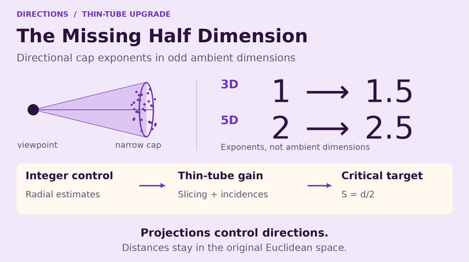
Stand at one endpoint and look toward the other portion of the set. Each pair determines a direction on a sphere. A cap is a small patch of that sphere, and a cap bound limits the mass pointing into it. Geometrically, this controls concentration inside thin tubes.
The proof targets directional exponent . It cannot assume every radial projection has a density relative to full spherical surface measure. When the source dimension is below the sphere’s dimension, that assumption would demand more dimensional spread than the source can provide.
Integer directional exponents come from radial integrability after projection into a suitable smaller space. Odd ambient dimensions introduce the remaining difficulty: half the ambient dimension is a half-integer. In three dimensions, for example, the desired exponent is 1.5 rather than one.
A thin-tube upgrade supplies the missing half dimension through slicing and planar incidence estimates. The integer endpoint of the angular gain requires a separate transverse-triple argument. Auxiliary spaces organize directions and incidences only. Every final distance remains measured in the original Euclidean space, so projection does not quietly replace the theorem with a different metric problem.
In five dimensions, the same issue appears as a target exponent of 2.5 after an integer starting exponent of two. The repeated half-dimensional gap is why the odd-dimensional preparation deserves its own argument, rather than being dismissed as a minor adjustment of the even-dimensional case.
7. Fourier Analysis Converts Directions Into Distance Control
A tube test controls directions clustered near a point of the sphere. A scalar projection test concerns a belt, a different geometric shape. Moving between these controls is an essential step in the Falconer distance conjecture Fourier analysis, not a change of terminology.
Lemma 6.3 combines spatial and angular ball bounds, both with exponent . On each dyadic frequency annulus, the resulting power is at the critical choice. Here B denotes the frequency scale. Summing annuli produces logarithmic growth rather than an uncontrolled positive power.
The subsequent distance-shell estimate uses stationary phase, which analyzes cancellation in rapidly oscillating integrals. It first produces an angular inner product. Cauchy–Schwarz bounds this by a positive energy with independent angular variables, allowing the graph estimate to pass control into finer spatial cells.
Angular Fourier modes also appear in the analysis of irrational triangular billiards, though the mathematical target differs. Here the goal is to prevent the distribution of distances from remaining concentrated on a zero-length set. The proof does not assume the original fractal measure already has Fourier decay.
8. A Two-Depth Potential Pays for the Recursion
At frequency , dyadic regularization sorts each measure into classes with controlled cell masses. A profile m records how those masses decay as spatial resolution increases. The excess above critical decay is:
The index n is a depth in the spatial subdivision. A positive excess indicates more decay than the critical baseline predicts. Different scale intervals can behave differently, so a single global dimension number cannot track every step of the proof.
The recursion alternates between positive counts of pairs with nearly equal distances and angular Fourier energies. Advancing to finer cells, shortening an interval, or converting between states can introduce losses. The paper controls these with a potential formed from two excess-profile values at sufficiently separated depths.
Why two? A transition may spend information near one end of the interval while leaving the other available. The separated pair lets the accounting change one depth without losing all its reserve. Transition costs are bounded by increases in this potential, and those increases telescope along recursive branches.
At entry, the construction locates a small level . The two-depth reserve is roughly twice that level, while the entry cost is at most roughly one. After controlling the remaining losses, a strictly negative Fourier-shell exponent survives.
This accounting is an explanatory analogy, not a numerical simulation. The reserve consists of exponents in inequalities, and the costs quantify how those inequalities weaken under each reduction. The proof must also bound the number of transitions and fix its error budgets before sending the frequency scale to infinity.
9. Why the Limiting Measure Gives Positive Length
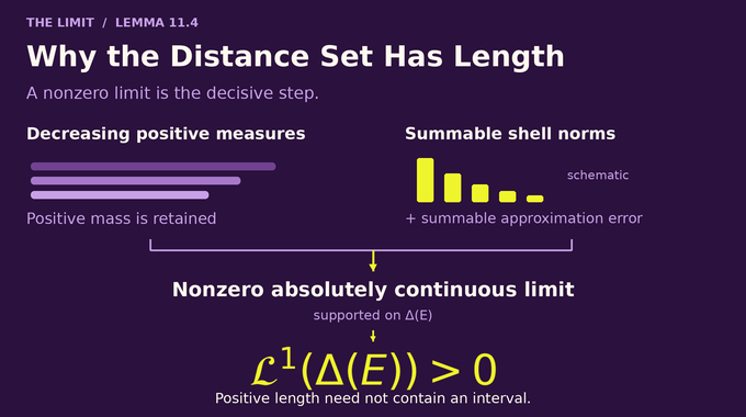
Frequency estimates must ultimately describe actual distances. The paper constructs decreasing positive distance measures and nearby approximants , whose Fourier transforms satisfy a decaying shell estimate:
The constant gamma is positive. Their total-variation discrepancy also decays geometrically, meaning the discarded mass is summable over scales. Crucially, the decreasing measures themselves need not approach their limit at a known quantitative rate.
Lemma 11.4 handles that gap. Positivity makes the successive differences of the decreasing measures summable, and telescoping smooth Fourier cutoffs reconstructs an absolutely continuous limit. The construction separately guarantees that this limiting measure is nonzero and supported on the original distance set.
An absolutely continuous measure gives zero mass to every zero-length set. Therefore, a nonzero such measure supported on the distance set forces that set to have positive length. Absolute continuity also matters in the Anderson localization research, but there it describes spectral measures. Here it describes a distribution of Euclidean distances.
The construction uses a positive distance-dependent weight. Because the two supports stay separated, that weight is bounded above and below by positive constants. It therefore preserves the essential conclusion that the limiting distance measure has positive mass. This prevents a formally smooth but empty limit from masquerading as a solution.
10. What the Lean Formalization Establishes
OpenAI’s Falconer formalization scope note identifies both an all-dimensional theorem and an earlier planar comparator. The comparator statements contain placeholders because they specify the verification targets. Reading those files alone does not assess the separate solution.
The all-dimensional solution module contains a theorem with the stated compactness, dimension, and positive-volume conclusion. Its proof invokes imported results and supplies the planar incidence input. The comparison configuration connects this solution module to the target statement.
This supports describing the repository as providing a formalization identified with the main theorem. It does not establish that the Lean development mirrors every page of the manuscript. The dependency tree and comparator were not rerun for this article, so this review does not independently certify that build.
As with formalizing Fermat’s Last Theorem, checking a formal statement and understanding its mathematical explanation are related but separate tasks. Neither a theorem name nor a successful compilation with unexamined assumptions would replace checking what was actually proved.
11. What Changes for Mathematics and AI Readers
The OpenAI Falconer distance conjecture proof targets a mathematical existence question. It supplies no demonstrated acceleration for nearest-neighbor search, embedding construction, point-cloud processing, or machine-learning training. A finite dataset has Hausdorff dimension zero, so applying the theorem directly to a sampled cloud would miss its hypothesis.
Its potential value lies in the analytical tools: improved directional concentration estimates, critical angular Fourier control, and a limiting-measure principle that tolerates unknown convergence rates. Whether those components produce further results requires additional mathematics.
OpenAI’s mathematics release announcement describes the wider AI-generated research program. That context explains provenance, while the theorem’s importance rests on its exact assumptions and conclusion. A result about all pairs does not automatically give one fixed point with a positive-length distance set.
The Falconer Distance Conjecture now has an all-dimensional proof presented at the sharp strict threshold, with supporting formalization identified in the public repository. Read it for the route from irregular geometry to positive length. Follow Binary Verse AI’s research-proof explainers for careful accounts of what each new mathematical result establishes, how its argument works, and where its evidence ends.
Has the Falconer distance conjecture been solved in every dimension?
OpenAI’s September 23, 2026 manuscript presents a proof for every integer : every compact set in with Hausdorff dimension greater than determines a distance set of positive Lebesgue measure. No additional structural regularity is assumed. The repository identifies a formalization of the main theorem. This describes the published claim and supporting artifacts, rather than asserting independent community acceptance.
Why is d/2 the critical threshold in Falconer’s conjecture?
Falconer’s lattice-based constructions give critical-dimensional sets whose distance sets have zero Lebesgue measure. Thus the strict threshold cannot be lowered in the general positive-measure statement. The manuscript proves its conclusion strictly above that threshold and makes no assertion at equality.
What is the difference between positive Lebesgue measure and a distance set of dimension one?
Positive Lebesgue measure means the distance set occupies a positive total length on the real line. Hausdorff dimension one alone does not guarantee this: a set can have full one-dimensional Hausdorff dimension and still have zero length. Positive length alone also does not guarantee that the set contains an interval.
How does OpenAI’s proof overcome the previous mathematical barrier?
The argument prepares directional cap bounds from Frostman measures, upgrades them through slicing and incidence geometry, and converts angular control into Fourier distance-shell estimates. A multiscale recursion uses a two-depth potential to control losses. A monotone-measure reconstruction argument then produces a nonzero absolutely continuous measure supported on the distance set.
Why are odd dimensions especially difficult in the proof?
For odd ambient dimension, is a half-integer. The initial directional preparation provides integer-dimensional cap control. A thin-tube upgrade supplies the remaining half dimension using slicing and incidence estimates. A separate transverse-triple argument handles the integer endpoint in the angular gain.
Does the Falconer distance conjecture proof also solve the pinned distance problem?
No. The theorem concerns all distances between pairs of points in the set. It does not establish that one fixed point in the set determines a positive-measure collection of distances at the same sharp threshold. The manuscript explicitly distinguishes its unpinned result from such a pinned conclusion.
Has OpenAI’s Falconer distance conjecture proof been formalized in Lean?
OpenAI’s scope documentation identifies a formalization of the main all-dimensional theorem and an earlier planar comparator. The separate all-dimensional solution module contains the stated theorem and invokes imported results. The comparator’s placeholders specify targets rather than the solution proof. This review did not compile the full development or rerun its comparator, and does not claim a line-by-line formalization of every argument in the 64-page manuscript.