
Randomness can trap a quantum particle. The harder question is whether weak randomness must trap it. The Anderson localization OpenAI proof addresses that second question: its September 23, 2026 manuscript establishes a nonempty energy interval with purely absolutely continuous spectrum for the nearest-neighbor Anderson model with independent uniform disorder, in every fixed dimension .
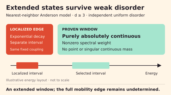
The interval stays fixed as disorder becomes sufficiently small. Its spectral weight is nonzero, and both eigenvalue mass and singular continuous mass are excluded there. That supplies the energy-range conclusion requested in Simon’s Problem 1 for this model. It does not locate the full mobility edge or prove quantum diffusion. The result’s substance lies in how the argument replaces artificial damping with genuine randomness without losing control.
Table of Contents
1. Anderson Localization OpenAI Proof: What Has Been Established?
The 93-page research manuscript proves a spectral statement about an infinite random lattice. It does not report a material experiment or a simulation speedup.
| Research Detail | Precise Scope |
|---|---|
| Lattice | Nearest-neighbor integer lattice , with fixed . |
| Randomness | Independent site potentials uniform on , multiplied by . |
| Disorder | Every fixed , for a dimension-dependent positive threshold. |
| Energy Window | Nonempty open interval , independent of disorder strength. |
| Conclusion | Almost-sure pure absolute continuity, with nonzero spectral weight. |
| Proof Status | Written preprint. The linked result #261 Lean note does not formalize this theorem. |
OpenAI’s mathematics release announcement attributes the collection to an internal frontier model. That establishes provenance. The mathematical evidence for this result is the manuscript’s argument, whose individual steps remain available for expert scrutiny.
2. The Anderson Model: How Random Potentials Change Quantum States
A wavefunction assigns a complex amplitude to each lattice site. The Hamiltonian combines hopping to adjacent sites with a random local energy:
Here is a site, its independent uniform random variable, and the disorder strength. Hopping has coefficient one, fixing the energy scale. The integer counts spatial directions. The negative hopping sign matches the paper’s convention.
Localization describes spectral states confined around particular regions, with exponentially decaying eigenfunctions in the localized regime discussed here. Absolutely continuous spectrum provides the spectral meaning of extended states used in this article. It does not specify a diffusion constant. Unlike the interacting spins in the quantum Heisenberg ferromagnet, this operator describes a single particle in a random landscape.
3. Simon’s Problem 1: Why Proving Delocalization in 3D Was So Difficult
Strong disorder and suitable extreme energies already admit rigorous localization methods. Reversing those arguments does not establish delocalization. To prove survival of extended spectral states, one must control the infinite-volume resolvent as its imaginary regulator vanishes, at a fixed positive coupling.
Tree models offer important precedents, but branching geometry differs from a Euclidean lattice with loops. A theorem on a tree cannot simply be transplanted onto a cubic grid. The geometry also matters in lattice percolation, although that problem concerns random connectivity rather than a quantum operator.
Earlier weak-coupling diffusion results take a different limit, with coupling tending to zero alongside changing time and space scales. Here the coupling is fixed before the boundary limit. As with the Haldane gap problem, strong physical evidence does not supply the missing uniform mathematical control.
The obstruction is visible in finite matrices: an inverse becomes sensitive when its energy approaches an eigenvalue. A positive imaginary regulator stabilizes it, but estimates that deteriorate as the regulator shrinks cannot establish the desired boundary statement. The new construction is designed to keep useful lower bounds throughout that limiting process.
4. Theorem 1.1: Purely Absolutely Continuous Spectrum at Weak Disorder
For three dimensions, fix a sufficiently small number . The theorem uses:
For higher dimensions, its interval is explicitly:
For every fixed , almost surely:
The first inclusion places the interval in the spectrum. The second says that projecting any square-summable state onto this energy window yields a state in the absolutely continuous spectral subspace. The projection is nonzero. This excludes an empty-window interpretation and rules out singular spectral mass throughout the restriction.
The probability-one event may depend on the fixed coupling. Constants may depend on dimension, without uniformity across all dimensions. The higher-dimensional threshold is defined through an infinite family of probability conditions on finite matrices, with no effective numerical bound. Three dimensions receive an existential positive threshold. These are existence guarantees, not calibrated laboratory disorder tolerances.
Spectral purity is stronger than detecting some extended contribution. A mixture of absolutely continuous and singular measures could still have an absolutely continuous component. The theorem excludes that mixture within its window. This is also a different question from a spectral gap, which asks whether an energy range contains spectrum at all.
5. The Finite-Volume Resolvent Certificate: The Foundation of OpenAI’s Proof
Proposition 2.1 moves the main construction onto a large periodic lattice, a finite grid with opposite faces identified. Its target is a modified inverse:
Here is the finite Hamiltonian, the selected energy, the active sites, and a positive scale tending to zero. The coefficients have bounded magnitude and imaginary parts bounded above and below by positive constants. The modification adds controlled complex damping only on active sites.
With probability approaching one as the construction scale grows, , where is the total site count, and every active diagonal imaginary resolvent entry stays bounded below. Crucially, the real potentials in the final finite Hamiltonian are the original true uniform variables. Auxiliary randomness helps find a certificate without changing that underlying disorder law.
A finite certificate therefore supplies a controlled route toward an infinite spectral conclusion. The Laughlin spectral-gap argument also uses certificates, but certifies a different property of a many-particle Hamiltonian.
6. Revealing Randomness One Binary Digit at a Time
Uniform disorder can be built from independent fair signs:
Each sign is plus or minus one with equal probability. Revealing successive signs installs progressively finer pieces of the true potential. The remaining unqueried tail is still uniform on a shrinking symmetric interval, conditional on the retained history.
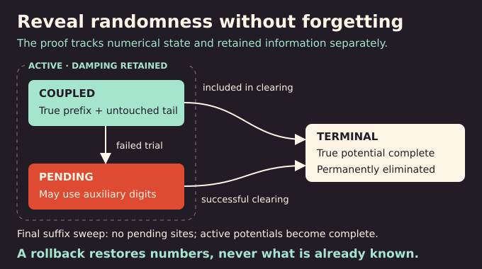
A coupled active site carries its true revealed prefix and an untouched suffix. A pending active site has lost that guarantee and may carry auxiliary digits. A terminal site has its complete true potential and is permanently eliminated from the active matrix.
Rollback restores numerical matrices, never knowledge. If a failed trial queried a digit, that answer remains recorded. Marking affected sites pending prevents later estimates from treating observed randomness as fresh. The conditional-freshness lemma justifies the remaining independent inputs, including at stopping times. This distinction is essential: forgetting a failed calculation is easy; making its information statistically disappear is impossible.
For example, if the first two signs at one site are plus and then minus, their installed contribution is one quarter of the disorder strength. The untouched remainder ranges uniformly between minus and plus that same quarter. Querying another tail digit changes what is known, even if its proposed numerical update is later rejected.
7. Schur Complements, Ward Identities, and the Laplacian Matrix
Schur complements remove terminal variables while exactly retaining their influence on surviving sites. The resulting damped inverse is , with rescaling . Two entrywise squares serve different purposes: retains complex phase, while is nonnegative.
Set and . The Ward identity gives:
The star denotes conjugate transpose. This identity turns resolvent amplitudes into an exact balance relation. It produces a graph Laplacian:
Its inverse quadratic form, defined on charges summing to zero, measures the accumulated spatial cost of updates. Separately, row fourth-power bounds prevent concentration on a few entries. The matrix controls linearization of the diagonal self-consistency equation through . These controls respectively protect spatial stability, distributed influence, and the ability to reset the diagonal.
Fourier estimates initialize them near the free band minimum. Dimensional dependence enters through these analytic estimates and spatial counting, rather than a slogan that particles simply have more escape routes.
8. Ordinary Sweeps: How the Proof Controls Each Random Update
An ordinary sweep trades part of the damping for one more digit of randomness. Algebraically, site splitting creates two ports, one for the inserted random contribution and one for the retained damping. Schur deletion then returns the calculation to its physical variables.
Updates are tested on finite tiles. Conditional concentration bounds monitor cumulative matrix changes, including the first update that would violate a bound. Local tests avoid paying for a union over the entire enormous lattice at every intermediate step.
When a trial fails, the matrices roll back, observed answers remain, and all active sites in that tile become pending. Retries use new auxiliary inputs. Accepted changes must still fit the global budgets. At stage end, a self-consistent reset restores .
The fixed-point reset is possible because its linearized operator is controlled. The broader finite-to-infinite issue also appears in the 2D area-law proof, where bounds must survive increasing system size. Here every sweep must preserve the estimates needed at smaller damping.
9. Clearing Pending Sites with Scattering Matrices and Projection Weights
Auxiliary digits cannot remain in the final operator. Small components of pending sites therefore undergo a separate clearing procedure. A symmetric unitary scattering matrix encodes interaction between a selected core and its exterior.
The range of its cross block identifies the exterior directions affected when the core is completed. A projection onto that range measures how much any such direction can concentrate at an individual surviving site. Small diagonal projection weights make the eventual completion harmless enough for the matrix budgets.
Regularized projection weights guide selection of exterior pivots, where untouched true residuals can be exposed. Spatial estimates control the whole scattering range even when some singular values are arbitrarily small. This avoids relying on an unjustified lower singular-value bound.
A negative-drift estimate bounds the number of exterior exposures, while stopped martingale estimates control their cumulative effects. After preparation succeeds, any unknown core values are revealed and installed. The core and exposed exterior sites become committed terminals. Failed clearings roll back provisional numerical changes and conservatively mark inspected sites pending. The procedure controls sensitive regions without assuming their already-observed values are independent again.
Think of the projection weight as a worst-case influence score, rather than an estimate for one convenient vector. Controlling the entire range protects against whichever core completion occurs. The regularization helps identify dangerous directions without assuming that a nearly invisible scattering direction can simply be discarded.
10. Failure Histories and Induction: Why the Construction Eventually Succeeds
A deterministic induction keeps committed changes within bounds, preserves geometric separation, and retains at least half the physical sites as active. A probabilistic induction shows that pending sites disappear with sufficiently high probability.
Every failure receives a chronological label. Conditional failure bounds multiply through successive conditioning for distinct specified labels. The argument does not assume the failures themselves are independent.
A surviving pending site must have a recent failure or many separated older witnesses. The history analysis ensures distinct leaf labels, preventing one old failure from being counted repeatedly as several independent pieces of evidence. Geometric counting then pays for the possible witness locations.
With high probability no pending sites remain at the cutoff and later sweeps succeed. A final true-suffix sweep installs all remaining genuine potentials while retaining small damping on active sites. The multi-scale organization invites comparison with the BKT transition argument, though its physical quantities and estimates differ.
The two inductions answer complementary questions. Deterministic estimates say that accepted operations preserve a valid state. Probability estimates say that the adaptive procedure reaches the required endpoint often enough. Neither statement substitutes for the other, and both must use the same retained history when deciding which randomness is still available.
11. Spectral Averaging: From Finite-Volume Bounds to Pure Absolute Continuity
The certificate concerns a specially damped finite inverse. Section 9 must transfer its information to the ordinary infinite-volume resolvent of the true operator. Comparison through a narrow-energy spectral projection controls the discrepancy using that projection’s rank.
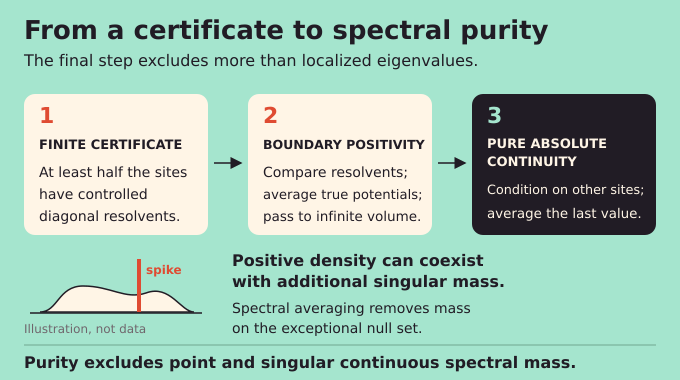
Averaging a site’s potential under the original product law bounds the expected rank. This yields positivity for a bounded function of the true diagonal imaginary resolvent, which passes to infinite volume. Ergodicity and rank-one comparisons propagate boundary positivity between sites at almost every fixed energy.
That is still insufficient for purity. A measure can have a positive density almost everywhere and additional singular mass on an exceptional null set. The paper conditions on every potential except one, constructs an exceptional energy set independent of that remaining variable, and applies own-site spectral averaging to remove its spectral mass.
The result excludes both eigenvalue and singular continuous contributions. This conversion of local conditional information into a global conclusion is also a useful reading theme in the Mézard–Parisi formula explainer, although its target is thermodynamic pressure.
For a state concentrated at one site, its spectral measure assigns weight to energy sets. Absolute continuity means that every set of zero ordinary energy length receives zero weight. Establishing this for all lattice basis states, then using density and closure, supplies the theorem for the entire projected spectral subspace.
12. What the OpenAI Proof Resolves and What Remains Open
Corollary 1.2 combines the result with existing edge localization: at the same fixed weak coupling, a separate interval near the lower spectral edge has localized eigenfunctions. Delocalization in the selected window therefore coexists with localization elsewhere.
| Question | Answer |
|---|---|
| All energies extended? | No. Only the stated interval has the pure absolute-continuity conclusion. |
| Complete mobility edge? | No. The full localization-delocalization boundary is not located. |
| Quantum diffusion? | No. Simon’s separate Problem 3 is not resolved. |
| Numerical weak-disorder threshold? | No effective numerical bound is supplied. |
| Headline theorem verified in Lean? | No such verification is supplied by the linked #261 scope note. |
The official Lean scope documentation for result #261 identifies a supporting two-dimensional spectral-set theorem. It does not formally verify this three-dimensional absolute-continuity result. Written proof, formal verification, and practical performance are separate evidence categories, a distinction developed in our Fermat formalization explainer.
No computational resource saving follows from this spectral theorem. Readers seeking that kind of evidence can compare the explicit circuit counts in our Claude quantum-circuits analysis. Here the advance concerns the mathematical classification of spectral states.
For readers evaluating Anderson localization OpenAI research, the useful next step is to follow the certificate through its retained-information rules and final spectral readout. That is where the proof earns its conclusion. Explore Binary Verse AI’s linked mathematical-physics explainers to compare what each theorem actually controls.
What does OpenAI’s Anderson localization proof establish?
OpenAI’s proof establishes that the nearest-neighbor Anderson model on the integer lattice, in every fixed dimension of at least three and for every fixed sufficiently weak positive independent uniform disorder strength, almost surely has a nonempty open energy interval with purely absolutely continuous spectrum and nonzero spectral weight. The interval may depend on dimension but is independent of disorder strength.
Why is Anderson localization different in three dimensions?
The distinction here concerns whether extended spectral states survive disorder. The paper establishes an absolutely continuous energy interval in three and higher dimensions using dimension-dependent Fourier and spatial estimates. It does not establish an equivalent result in one or two dimensions.
What does purely absolutely continuous spectrum mean?
It means that the spectral measures restricted to the selected energy interval are absolutely continuous with respect to Lebesgue measure. The restriction therefore contains neither pure-point spectral mass nor singular continuous spectral mass.
How does OpenAI’s proof overcome the previous mathematical barrier?
The proof constructs a finite-volume resolvent certificate while revealing independent disorder incrementally. Ward identities, matrix bounds, controlled trials, and probabilistic failure estimates preserve the required controls. A final comparison and spectral-averaging argument transfer them to the true infinite-volume operator and establish spectral purity.
Does the proof show that all quantum states in 3D are extended?
No. The theorem establishes purely absolutely continuous spectrum only on a specified nonempty open energy interval. A separate interval near the spectral edge has localized eigenfunctions at the same fixed weak disorder strength, by the paper’s coexistence corollary and the existing localization result it invokes.
Does OpenAI’s proof determine the Anderson mobility edge or prove quantum diffusion?
No. It establishes an absolutely continuous energy interval without determining the complete boundary between localized and delocalized spectral regions. It also does not resolve the separate diffusion question stated as Simon’s Problem 3.
Is OpenAI’s Anderson localization proof verified in Lean?
The official Lean scope note for result #261 describes a supporting theorem identifying the almost-sure spectral set of a two-dimensional Anderson operator. It does not formally verify the headline theorem on purely absolutely continuous spectrum in three and higher dimensions.