
Physicists have spent decades confidently describing an energy gap that mathematicians couldn’t rigorously guarantee for the simplest model behind it. The evidence was strong. The missing step was proving that the gap survives however long the quantum chain becomes.
OpenAI’s September 24, 2026 manuscript, The periodic spin-one Haldane gap, presents a proof of that claim for even periodic spin-one Heisenberg chains. Released in its October mathematics collection, the paper addresses a central formulation of the Haldane gap conjecture, published in 1983. OpenAI announced the collection on October 6.
The claimed advance is specific: a unique ground state for sufficiently large even rings, with a positive excitation gap bounded below independently of their length. It doesn’t determine the gap’s exact value or settle every spin and boundary condition.
The intriguing part is the route. The argument connects two ways of describing the same thermal system, then repeatedly sharpens finite estimates until they control arbitrarily long chains. Understanding that mechanism matters more than simply declaring a forty-three-year problem finished.
Table of Contents
1. Haldane Gap Conjecture: What Did OpenAI Actually Prove?
The paper studies the pure antiferromagnetic spin-one Heisenberg model, with nearest-neighbor interactions and periodic boundaries. Its main theorem supplies explicit lower bounds on the energy needed to leave the ground state.
Haldane Gap Conjecture: Key Manuscript Claims and Gap Bounds
| Key Fact | What the Manuscript States |
|---|---|
| Model | Pure bilinear spin-one Heisenberg chain, coupling set to one |
| Geometry | Even periodic rings |
| Ground State | Unique for every even length L ≥ 60 |
| First Gap Bound | γL > (4/105) log(80/79) for even L ≥ 60 |
| Stronger Bound | γL > log(20)/784 for even L ≥ 2304 |
| Large-System Conclusion | Positive lower limit of the gaps as even lengths grow |
The original research paper is available in OpenAI’s repository. Calling its argument a proof describes the manuscript’s mathematical claim. Independent acceptance requires checking the construction, finite certificates, and deductions.
OpenAI itself says the collection contains results at different verification stages and warns that unformalized results may contain issues. That disclosure applies to interpreting the release, without establishing whether this particular argument is correct.
2. Why Haldane’s Prediction Was So Surprising
Spin is intrinsic quantum angular momentum. In this model, each spin-one site has three local basis states. Neighboring spins interact antiferromagnetically, favoring opposite alignment, although the quantum ground state isn’t simply a row of alternating arrows.
Haldane’s conjecture distinguished integer-spin chains from half-integer-spin chains. The surprise was qualitative: changing the spin could change whether excitations require a finite minimum energy in the infinite-chain limit.
His continuum argument connected the chain to the (O(3)) nonlinear sigma model, with a topological term that distinguishes the two spin classes. This field-theory description supplied a compelling physical explanation, but establishing the lattice model’s spectral gap still required a rigorous argument.
Haldane Gap Conjecture: Gapped Chains, Spin Types and Boundary Effects
| Concept | Practical Meaning | Important Qualification |
|---|---|---|
| Gapped Chain | Excitations cost a minimum positive energy | The minimum must survive increasing length |
| Gapless Chain | Excitation energies can approach zero | A finite sample can still show separated levels |
| Integer Spin | Haldane predicted gapped antiferromagnetic chains | This paper specifically treats spin one |
| Half-Integer Spin | Different low-energy behavior is expected | Rigorous obstructions allow ground-state degeneracy |
| Open Boundaries | End spins can introduce low-energy states | A periodic-ring theorem doesn’t automatically cover them |
The prediction was first formulated in 1981 and published in 1983. The familiar forty-three-year description counts from publication to 2026.
3. The Hamiltonian: A Simple Formula With a Difficult Spectrum
The model is defined by
[ H_L=\sum_{j=0}^{L-1}\mathbf S_j\cdot\mathbf S_{j+1}, \qquad \mathbf S_L=\mathbf S_0. ]
The last equality closes the chain into a ring. Each term couples neighboring spin operators, and the interaction strength is normalized to one.
Write (E_0(L)) for the lowest energy and (E_1(L)) for the next distinct energy. The finite-chain spectral gap is
[ \gamma_L=E_1(L)-E_0(L). ]
A positive gap for one finite chain is insufficient. For example, a sequence of gaps behaving like (1/L) stays positive at every finite length while approaching zero. The spin-1 Heisenberg chain spectral gap must instead have a positive lower bound that doesn’t shrink away.
This is where the problem becomes demanding. The Hilbert space has dimension (3^L), so directly inspecting larger matrices soon becomes impractical. Even perfect calculations for many lengths leave infinitely many unchecked. The proof needs a rule that reaches beyond its computed examples.
4. Why the Gap Resisted Proof for Decades
The spin-1 Haldane gap had substantial numerical and experimental support. White and Huse’s density-matrix renormalization-group study estimated the bulk gap as approximately (0.41050). Experiments on the nearly one-dimensional antiferromagnet CsNiCl₃ supported the physical picture.
Those results answered important physics questions. They didn’t provide an inequality valid for every sufficiently large chain.
The Affleck–Kennedy–Lieb–Tasaki, or AKLT, model offered another major advance: a rigorously gapped spin-one chain with an explicit ground-state construction. Its interaction includes a biquadratic term, proportional to ((\mathbf S_j\cdot\mathbf S_{j+1})^2). The pure Heisenberg chain lacks that term.
Proving stability near the AKLT interaction doesn’t automatically extend the gap all the way to the pure bilinear model. The path between two interactions needs its own control.
Standard finite-size gap criteria also often depend on frustration-free structure, where the ground state minimizes every local interaction simultaneously. Those tools don’t directly settle this model. A Haldane gap conjecture proof therefore needed more than another convincing extrapolation or a nearby solvable chain.
5. What the Main Theorem’s Bounds Mean
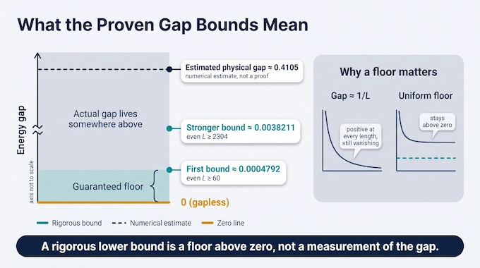
The first bound is approximately (0.0004792). The stronger eventual bound is approximately (0.0038211), giving
[ \Delta_1:=\liminf_{\substack{L\to\infty\L\text{ even}}}\gamma_L \ge\frac{\log20}{784}>0. ]
These numbers are much smaller than the estimated physical gap of (0.4105). That isn’t a contradiction. A rigorous lower bound certifies a floor, rather than identifying the actual excitation energy. The theorem’s decisive feature is that its floor remains above zero.
The manuscript also separates ground-state uniqueness from a gap above the ground-energy sector. Its explicit uniqueness statement begins at even (L=60). The finitely many smaller even chains have positive gaps above their ground sectors, but this observation supplies neither the stated numerical bounds nor a uniqueness claim for those lengths.
Those qualifications are part of Theorem 1.1 and its accompanying discussion. Haldane gap conjecture(1).pdf
The OpenAI Haldane gap proof thus targets the central existence question. It doesn’t claim a precise new measurement of the gap.
6. One Partition Function, Two Representations
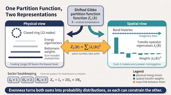
The central construction starts with a shifted Gibbs partition function,
[ Z_L(b)=\operatorname{Tr}\exp[-b(H_L+aLI)], ]
where (b>0) is inverse temperature and (a) is a scalar energy shift. Increasing (b) cools the system, giving lower-energy states greater relative weight. The shift changes the normalization without changing energy differences.
Physically, this trace sums positive Boltzmann weights over all energy eigenvectors, including their multiplicities.
The paper constructs a second representation using a self-adjoint spatial transfer operator. Its eigenvalues (\lambda_i(b)) satisfy, for even lengths,
[ Z_L(b)=\sum_i|\lambda_i(b)|^L. ]
The operator acts on bond histories, lists recording interaction events along imaginary time. These auxiliary objects encode the same partition function in the spatial direction.
Evenness does real work here. Transfer eigenvalues can be negative, but even powers are nonnegative. Both representations therefore produce probability distributions. The spatial eigenvalues aren’t the physical energy levels, and confusing them would erase the point of the construction.
7. How Twists and Rotations Expose the Dominant Weight
Small partition-function calculations alone don’t identify which transfer weights dominate. The proof gains information by temporarily twisting the interaction across the ring’s closing bond.
These twists are auxiliary calculations. The final theorem concerns the untwisted Hamiltonian.
Rotations by (\pi) about the coordinate axes form the (D_2) symmetry group used in the argument. A cyclic rotation also permutes the three axes. Together, these symmetries separate transfer eigenvalues into sectors with controlled multiplicities.
The sector moments enter the ordinary partition function as
[ Z_n=I_n+2O_n+3N_n. ]
Twisted traces supply different combinations of the same moments, allowing the proof to bound them separately. Every weight outside the jointly invariant sector occurs at least twice in the full transfer spectrum.
That multiplicity becomes a useful restriction: strong enough concentration cannot hide in a repeatedly occurring weight. The argument uses the sector bookkeeping to identify a single dominant spatial contribution while retaining the complete spectrum.
8. Physical Purity and Spatial Purity
Purity measures concentration. For probabilities (p_i), it is (\sum_i p_i^2). A distribution concentrated on one outcome has purity one. Two equally likely outcomes have purity one-half.
Here, purity is a mathematical diagnostic, with two distinct roles.
Consider probabilities (0.9) and (0.1). Their purity is (0.82). Squaring and renormalizing changes them to (81/82) and (1/82), raising purity to about (0.976). The favored outcome rapidly absorbs almost all the mass. The proof turns this simple concentration effect into quantitative estimates for much larger distributions, with their full multiplicities included.
8.1. Spatial Purity Measures Transfer-Weight Concentration
The spatial probabilities are (|\lambda_i(b)|^n/Z_n(b)). Their purity is
[ S(n,b)=\frac{Z_{2n}(b)}{Z_n(b)^2}. ]
Squaring and renormalizing these probabilities replaces length (n) with (2n). One dominant transfer weight becomes more dominant as the spatial moment increases.
8.2. Physical Purity Measures Thermal-State Concentration
The normalized Boltzmann weights have purity
[ T(n,b)=\frac{Z_n(2b)}{Z_n(b)^2}. ]
Squaring physical weights doubles inverse temperature. Cooling concentrates the distribution toward the lowest-energy eigenvectors.
Both ratios involve the same partition functions, giving exact cancellation identities, including
[ S(n,2b)=S(n,b)^2\frac{T(2n,b)}{T(n,b)^2}. ]
A complementary identity expresses (T(4n,b)) through spatial and physical purities. These relationships let progress in one distribution constrain the other. The bridge is algebraically exact, rather than an assumed similarity between space and temperature.
9. The Doubling Argument That Reaches Every Larger Chain
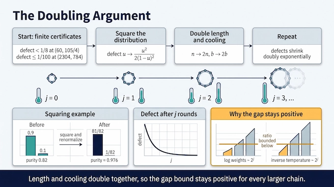
The proof’s elementary engine is a squaring lemma. If a distribution has small purity defect (u=1-P), its normalized squared distribution has defect bounded by
[ f(u)=\frac{u^2}{2(1-u)^2}. ]
For small (u), the improvement is quadratic. A modest initial concentration can become extremely sharp after repeated squaring.
Proposition 4.3 combines this observation with the cancellation identities. Its starting inputs are spatial purity at length (n_0) and physical purity at length (2n_0), at a common inverse temperature. Their different lengths matter.
The coupled update doubles the base length and inverse temperature together. Once the required thresholds hold, both defects decay doubly exponentially with the iteration number.
This scaling is what produces a uniform energy bound. Taking logarithms of the shrinking excited-state weights produces a factor growing like (2^j). Inverse temperature also grows like (2^j), so their ratio stays bounded below.
The result reaches arbitrarily large lengths without diagonalizing arbitrarily large Hamiltonians.
Cooling a fixed finite system would already concentrate its thermal weights, even if its gap were tiny. The harder achievement is controlling concentration while length grows too. The spatial purity supplies that missing control. Without the coupled estimates, low-temperature concentration by itself wouldn’t rule out a gap that vanishes as the system becomes larger.
10. Finite Certificates: Where Computation Enters
The Haldane gap conjecture argument still needs verified starting conditions. Its appendices provide finite thermal calculations at inverse temperatures (21/2) and (49/4), together with variational energy estimates.
The thermal inputs are bounds on matrix-exponential traces for short twisted chains. They use integer arithmetic, rational intervals, and explicit truncation errors. A floating-point eigenvalue estimate isn’t taken as a proof premise.
Polynomial filters restrict possible spatial eigenvalues using known moments. A nonnegative polynomial would contribute too much to those moments if an eigenvalue lay outside an allowed range, creating a contradiction.
Matrix-product trial states supply upper bounds on ground-state energies at lengths 72 and 120. A trial state needn’t be the exact ground state to give a rigorous variational bound.
Together, these inputs establish two initialization regimes: purity defects below (1/8) at a base pair ((60,105/4)), and at most (1/100) at ((2304,784)).
The longer initialization is reached through bounded updates from shorter inputs. Computation supplies the starting certificates, while the analytic argument explains why they remain useful beyond the computed sizes.
11. From Concentration to a Spectral Gap
Repeated doubling covers selected lengths. Spatial moment inequalities fill the intervals between them, controlling every intermediate even length rather than leaving gaps in the argument.
The final step returns to physical Boltzmann probabilities. Once physical purity exceeds one-half, the largest individual probability exceeds one-half too.
Two ground-state eigenvectors would have equal maximal Boltzmann weights. They couldn’t both carry more than half the total probability. This proves ground-state uniqueness in the theorem’s range.
For a ground-state weight (w_0) and a first-excited eigenvector’s weight (w_1),
[ \frac{w_1}{w_0}=e^{-b\gamma_L}. ]
Controlling this ratio yields the spectral-gap inequality.
Corollary 6.1 also passes the lower bound to local excitations in subsequential thermodynamic limits of periodic ground states. This supports an infinite-chain interpretation, but the argument doesn’t establish that every subsequence produces the same state or prove uniqueness among all infinite-volume ground states.
12. What Is Settled, What Still Needs Checking, and Why It Matters
For readers searching “Haldane conjecture solved,” the precise answer is that OpenAI presents a proof of the positive even-periodic spin-one formulation. It doesn’t establish every integer-spin case, arbitrary boundary conditions, or the exact gap value.
A separate boundary-field companion paper addresses odd open chains with endpoint field (h=3/5). OpenAI’s overview states that it also constructs boundary-selected infinite-volume states with topological index (-1). Those conclusions require that companion’s additional argument.
As of October 11, 2026, completed independent verification of this specific theorem hasn’t been established by the sources reviewed for this article. OpenAI’s general formalization statistics cannot certify an individual paper.
The main checkpoints are the identity linking physical traces to spatial moments, the error bounds in the finite trace calculations, and the threshold inequalities that start the iteration. Verifying only the final displayed gap inequality wouldn’t validate its inputs. These are specific mathematical claims that other researchers can examine and reproduce.
The research contribution to examine is concrete: a transfer representation, two coupled purity estimates, and finite certificates that propagate to every larger even ring. If validated, this would close a major gap between physical confidence and mathematical control.
Read the original theorem and Proposition 4.3 together, then check the appendices that initialize the argument. Follow Binary Verse AI for research explainers that track the Haldane gap conjecture from its stated proof to independent scrutiny, with the mathematics kept in view.
1. What does the Haldane gap conjecture state?
The Haldane conjecture predicts fundamentally different low-energy behavior for integer-spin and half-integer-spin antiferromagnetic Heisenberg chains. In particular, the spin-1 chain should have a nonzero energy gap separating its ground state from excited states, even in the infinite-chain limit.
2. Did OpenAI prove the Haldane gap conjecture?
OpenAI’s September 2026 paper presents a proof of the spin-one Haldane conjecture for even periodic chains. It establishes a unique ground state for every even length \(L\ge60\) and a strictly positive spectral gap uniformly bounded below as chain length increases. It does not prove every possible formulation of the conjecture.
3. Why was the Haldane gap conjecture so difficult to prove?
Numerical calculations and experiments strongly supported the gap, but they could not establish a rigorous lower bound for arbitrarily long chains. Earlier rigorous results, notably the AKLT model, concerned a Hamiltonian containing an additional biquadratic interaction. Proving the corresponding result for the pure spin-1 Heisenberg Hamiltonian remained a separate obstacle.
4. How does OpenAI’s Haldane gap proof work?
The proof represents the same partition function through physical energy levels and a spatial transfer operator. It then couples two probability-purity estimates, which improve through repeated doubling of chain length and inverse temperature. Rigorously certified finite calculations initialize the argument, while interpolation and Gibbs-weight inequalities establish a uniform positive gap for all sufficiently large even chains.
5. Has OpenAI’s Haldane gap proof been independently verified?
As of October 11, 2026, the paper provides explicit finite computational certificates and a complete written mathematical argument, but I could not confirm comprehensive independent verification or a full Lean formalization of this particular result. These are separate questions from whether the claimed argument is mathematically correct.