
A mathematical question can survive 126 years not because nobody knows how to count, but because nobody knows whether the counting can ever get out of control. That is the tension behind Hilbert’s 16th Problem, and it sits at the center of a striking new OpenAI manuscript.
Released in OpenAI’s October 2026 mathematics collection and dated September 24, Uniform Bounds for Planar Polynomial Limit Cycles claims to establish something mathematicians had not proved: for any fixed polynomial degree, there is a finite ceiling on the number of isolated repeating trajectories a planar system can have.
So, has Hilbert’s 16th Problem been solved? The paper claims to settle the uniform boundedness assertion in its second part. It does not calculate that ceiling, classify all possible cycles, or settle the separate algebraic-curve problem. The general proof is also not covered by the companion Lean formalization. Its significance would be enormous if its 160 pages withstand independent scrutiny. Here is what the argument actually says.
Table of Contents
1. Hilbert’s 16th Problem Solved? The Claim at a Glance
| Question | What the September 2026 Paper Says |
|---|---|
| What is claimed? | A finite upper bound exists for limit cycles at every fixed polynomial degree. |
| What systems qualify? | Real polynomial vector fields in the plane, with unrestricted coefficients, cycle locations, and stability. |
| What is the new method? | Complex asymptotic separation, controlled passage maps, and finite-dimensional counting. |
| Does it give a number? | No effective formula for the degree-dependent bound is supplied. |
| Is the general result Lean-verified? | No main-theorem formalization is listed in OpenAI’s Lean scope notes. |
| What remains? | Exact maxima, cycle configurations, explicit bounds, and independent proof assessment. |
This is not a numerical breakthrough of the form “degree five permits exactly N cycles.” It is an existence claim: however wildly the coefficients change, fixing the degree should prevent the number of limit cycles from growing without limit.
2. What Did Hilbert’s Original Sixteenth Problem Ask?
In 1900, David Hilbert presented problems intended to guide future mathematical research. His sixteenth was effectively two major questions sharing an interest in shapes and arrangements.
The first concerns the topology of real algebraic curves, including how their oval components can sit relative to one another. The second asks about the number and placement of limit cycles in polynomial differential equations on the plane.
The OpenAI paper concerns the second question only. A headline suggesting that every aspect of Hilbert’s original problem has been classified would be misleading. Its specific target is a necessary preliminary question: can a fixed-degree polynomial system support an unlimited number of isolated closed trajectories as its coefficients vary?
3. What Are Limit Cycles in Planar Polynomial Systems?
Start with a point moving across a plane. Its velocity is set by two polynomial functions:
[
\dot{x}=P(x,y),\qquad \dot{y}=Q(x,y).
]
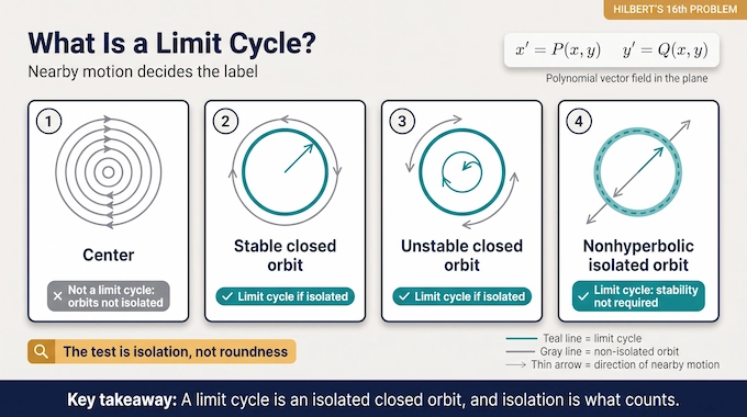
Together they define a vector field, a rule specifying the direction and speed of motion at each location. A trajectory might head toward a stationary point, spiral away, or close into a loop. When a closed trajectory is isolated from other periodic trajectories, it is a limit cycle.
Consider a ring that attracts nearby trajectories. A point starting slightly inside spirals outward toward the ring. One starting outside spirals inward. Both approach the same repeating orbit. That is a stable limit cycle.
| Motion Pattern | What Nearby Paths Do | Counts as a Limit Cycle? |
|---|---|---|
| Center with nested closed orbits | Nearby paths also form closed loops. | No. The periodic orbits are not isolated. |
| Stable closed orbit | Nearby paths approach the loop. | Yes, if it is isolated. |
| Unstable closed orbit | Nearby paths move away from the loop. | Yes, if it is isolated. |
| Nonhyperbolic isolated orbit | Motion close to the loop has more delicate behavior. | Yes. Stability is not a requirement. |
Conceptual picture: A center resembles many concentric circular tracks, each a possible periodic orbit. An isolated limit cycle resembles one distinguished circular track with neighboring motion that does not close into other nearby tracks. The difference is isolation, not whether the picture looks circular.
4. Why the Previous Mathematical Barrier Was So Difficult
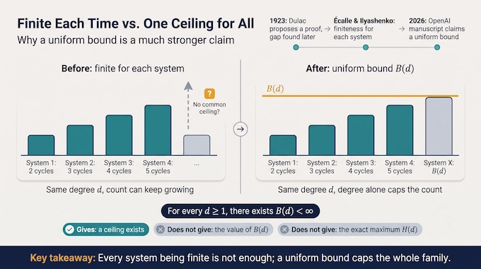
Mathematicians already had a finiteness theorem for each individual polynomial vector field. Henri Dulac proposed a proof in 1923, but a gap was later identified. Work by Jean Écalle and Yuri Ilyashenko established individual finiteness through sophisticated analysis of return maps.
But individual finiteness does not imply uniform boundedness. Imagine infinitely many systems of the same degree: the first has two cycles, the next three, then four, and so on. Each system still has finitely many. Across the family, however, there would be no common ceiling. That is the logical gap the new paper seeks to close.
Earlier advances controlled important restricted situations. Bautin’s result concerns cycles emerging near certain quadratic singularities. Studies of elementary polycycles and generic parameter families produced cyclicity bounds. The infinitesimal version of Hilbert’s question yielded constructive results involving Abelian integrals. None automatically covered every possible degeneration across all coefficients.
Equilibria can lose ordinary regularity. Trajectories can pass through neighborhoods governed by vastly different scales. Cycles may drift arbitrarily far from the origin. A method that counts ordinary, well-behaved cycles is not enough if exceptionally delicate ones escape its assumptions.
5. OpenAI’s Main Theorem: What a Uniform Bound Really Means
Theorem 1.1 of the OpenAI manuscript states that for every integer degree (d\geq1), there is a finite integer (B(d)) so that every real planar polynomial vector field of degree at most (d) has no more than (B(d)) limit cycles across the entire plane.
[
\forall d\geq1,\ \exists B(d)<\infty:\quad N_{\mathrm{cycles}}(P,Q)\leq B(d).
]
Notice the order of the words for every degree and there exists a bound. The bound depends on the degree, not on which coefficients someone chooses afterward. No upper limit on coefficient size is imposed. Neither is the result confined to a convenient square, to attracting cycles, or to generic systems.
The paper does not supply a practical algorithm for computing (B(d)). An existence theorem can rule out entire classes of hypothetical counterexamples without telling researchers the sharp numerical answer.
6. From Closed Trajectories to Zeros of a Return Map
The argument begins with a classical idea. Place a short transverse line across a periodic trajectory. Start near the point where the orbit crosses it, follow the differential equation through one circuit, and record where the trajectory next meets the line.
This creates a Poincaré return map, written (\Pi(r)), where (r) marks a starting position on the short line. If the trajectory returns to the same position, then (\Pi(r)=r). Consequently, neighboring limit cycles correspond to isolated zeros of the displacement function:
[
D(r)=\Pi(r)-r.
]
A simple zero has (\Pi'(r)\neq1) and represents a hyperbolic periodic orbit.
The return map can be assembled from passages near singular points where ordinary approximations break down. A zero-counting result for one fixed return map does not automatically apply uniformly to the entire family.
OpenAI’s proposed strategy is to replace the uncontrolled-looking collection of return maps with a carefully defined analytic class and a finite geometric description, then establish a uniform way to count its relevant solutions.
7. Proof Step One: Separating Asymptotic Packets
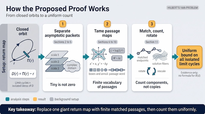
Sections 2 through 5 supply the most abstract part of the proposed proof. They study functions that arise when variables grow or shrink at dramatically different rates. A logarithmic flag records these ordered scales and their exact dependencies, so the argument can distinguish what dominates what as a system degenerates.
The next tool is an asymptotic packet. Rather than treating a formal expansion as though it automatically determines a function, the paper associates an actual analytic function with structured expansions, complex domains, and quantified error estimates. Two lateral sets of expansion data are compared as one moves through nested complex regions.
Why insist on complex domains? A function can become smaller than every algebraic power along a real path without being identically zero. Merely observing that an expression is extremely small is not enough to declare it absent. The manuscript’s separation theorem aims to promote suitably controlled asymptotic information into a genuinely decisive test of vanishing.
Next comes differentiated implicit calculus, used to change variables while preserving the delicate scale relationships. Finally, the authors formulate absolute isolated-zero finiteness for the particular analytic systems needed later. Roughly, if a supposedly isolated solution escaped through ever-larger scales, the constructed local charts would retain a free direction. That would conflict with isolation.
8. Proof Step Two: Taming Degenerate Passage Maps
Sections 6 through 8 test whether the actual passage maps of the differential equations meet the analytic requirements. The paper develops separate models for additive passages, relatively regular or stable passages, and situations involving two logarithmic scales.
Its simple saddle example shows why multiple clocks appear. For the system (\dot{x}=x), (\dot{y}=-\lambda y), the time needed to pass near the saddle involves (L=\log(1/r)). Another relevant quantity is (W=\lambda L). As (r) and (\lambda) shrink, one quantity may explode while the other stays moderate. One expansion cannot safely pretend those regimes are interchangeable.
The manuscript keeps track of small correction terms, including exponentially tiny contributions that could still affect the detection of a zero.
Sections 9 and 10 then move from analysis back to geometry. Polynomial vector fields of bounded degree are subdivided into finitely many prepared regions, including boxes and annuli. Local trajectories become sequences of passage types, or passage words. A crossing argument for closed planar orbits bounds the complexity of those words.
Without that uniform finite vocabulary, controlling each local passage would still leave an unlimited number of ways to assemble a complete orbit.
9. Proof Step Three: Matching Equations, Counting, and Rotation
Section 11 is where the analytic machinery is meant to pay off. Instead of composing every difficult passage map into one gigantic expression, the authors write matching equations that require consecutive passages to connect correctly. A closed trajectory corresponds to a consistent system of matched endpoints.
An isolated periodic orbit still has multiple representations, because the chosen cut points can slide along it. The paper accounts for this by studying connected components of solution fibers, rather than naively counting every solution as a different cycle. Its projection-counting theorem is then used to derive a uniform bound on those components for the permitted analytic systems.
Initially, this gives control over hyperbolic cycles in a fixed region. Two final moves broaden the result. A small signed rotation of the vector field is argued to create at least as many hyperbolic cycles near any finite collection of isolated cycles, while preserving polynomial degree. Then a spatial rescaling puts any chosen finite collection of cycles inside the fixed region.
Otherwise, an alleged bound could miss cycles drifting beyond the observation window or cycles too degenerate to be hyperbolic. In the manuscript, the rotation and rescaling argument connects the technical counting result to all isolated limit cycles in the plane.
10. What Remains Unsolved: Hilbert Numbers and Cycle Arrangements
There are two different mathematical quantities here. (B(d)) is any valid uniform upper bound. The Hilbert number (H(d)) is the largest number of limit cycles that a degree-(d) planar polynomial system can realize, assuming a finite maximum exists. A theorem showing that some (B(d)) exists need not identify (H(d)).
For instance, known constructions establish at least four limit cycles for quadratic systems and at least thirteen for cubic systems. Those are lower bounds: concrete examples show that many cycles are possible. They don’t say no system can have more. Research improving lower bounds and research proving upper bounds push from opposite directions.
Even the exact quadratic Hilbert number remains unknown. The algebraic-curve component of Hilbert’s original problem is a separate subject.
The broader mathematical payoff is therefore conceptual. If the uniform-boundedness claim survives scrutiny, one longstanding question becomes a foundation on which sharper questions can be built. Calculating effective bounds, determining exact maxima, and understanding allowable arrangements would remain ambitious programs in their own right.
11. What Has Been Verified, and What Must Mathematicians Check?
A second OpenAI manuscript, Two Limit Cycles for Quintic Liénard Systems, concerns a restricted family with equations (x’=y-F(x)) and (y’=-x), where (F) has degree at most five. OpenAI’s Lean scope documentation says its formalized theorem gives an upper bound of two limit cycles in that family and an example attaining two.
That is an exact answer for a specified class. It is not an exact answer for all degree-five planar polynomial equations, and it is not a Lean verification of the general uniform-bound theorem. A repository label marking the broader research family as having Lean material can be misleading unless readers inspect the formal statement itself.
A proof assistant checks formal deductions against a formal statement and its dependencies. Independent validation must also confirm that the formal statement expresses the intended mathematical theorem, that the assumptions are appropriate, and that any unformalized manuscript argument is sound. For the main 160-page proof, expert checking of the analytic separation, passage reductions, parameter uniformity, and projection-counting interface is especially important.
Publication on a repository, however, is not a substitute for detailed external review. As of October 10, 2026, the sources reviewed here do not establish that the full general proof has passed such an audit.
12. Why This Result Matters, and What to Watch Next
The significance of Hilbert’s 16th Problem is not that we might soon have a button that counts all oscillations in a model. The manuscript supplies no such tool. Its importance is the proposed transition from “every individual system has finitely many cycles” to “the degree alone limits the number across every system.” That is a much stronger statement about what polynomial dynamics can do.
Generating a sophisticated argument is an achievement of one kind. Making that argument legible, independently reproducible, and ultimately trustworthy is another. Mathematics does not waive the second requirement because the first is impressive.
Read the original paper, compare its Section 11 conclusion with the published Lean scope, and follow Binary Verse AI for research-first explainers that separate the theorem, the proposed proof, and the evidence behind the headlines.
1. Has OpenAI solved Hilbert’s 16th problem?
OpenAI’s September 2026 paper claims to establish the uniform boundedness assertion in the second part of Hilbert’s 16th problem. It proposes that planar polynomial systems of any fixed degree have a finite maximum number of limit cycles. However, the result does not determine the exact maxima or resolve every aspect of Hilbert’s original problem. The main proof also requires independent mathematical verification before its correctness can be regarded as established.
2. What is a limit cycle in Hilbert’s 16th problem?
A limit cycle is an isolated closed trajectory of a dynamical system, representing motion that repeats periodically. Isolation means there are no other periodic orbits sufficiently close to it. Unlike an ordinary periodic orbit, which may belong to a continuous family of closed trajectories, a limit cycle stands apart from neighboring periodic motion. Its stability does not determine whether it counts.
3. Why was Hilbert’s 16th problem so difficult to solve?
Earlier mathematicians established finiteness of limit cycles for individual planar polynomial systems, but this did not give a common upper bound for every system of the same degree. Changing polynomial coefficients can produce complicated degenerations, interacting trajectories, and cycles escaping toward infinity. OpenAI’s proposed proof addresses these obstacles using complex asymptotic analysis and finite-dimensional counting methods.
4. Does OpenAI’s proof give the exact maximum number of limit cycles?
No. The paper claims that for every degree \(d\), a finite upper bound \(B(d)\) exists, but it does not provide an effective formula or calculate the exact maximum, commonly denoted \(H(d)\). Even for quadratic polynomial systems, the exact maximum remains unresolved. Establishing that a finite maximum exists is mathematically different from determining its numerical value.
5. Has OpenAI’s Hilbert’s 16th problem proof been verified in Lean?
The main uniform-boundedness manuscript has no listed Lean formalization of its central theorem. OpenAI’s published Lean documentation instead covers a companion result proving that a specified family of quintic Liénard systems has at most two limit cycles, with examples attaining two. That formalization does not establish the general theorem for polynomial systems of arbitrary degree. Independent review of the main proof remains important.