
Must a graph comparison become polynomially harder as its dimension grows, or could a clever algorithm bypass the expensive refinement? OpenAI’s September 25, 2026 paper on unconditional WL lower bounds answers this question about weisfeiler leman time complexity. For every sufficiently large fixed dimension, every correct deterministic sequential decider needs an exponent proportional to that dimension in the worst case, at every sufficiently large graph size. This holds even for connected graphs of diameter at most two. The result concerns deciding WL equivalence, rather than merely running its familiar algorithm. It appears in OpenAI’s mathematics research release.
Table of Contents
1. What Is Weisfeiler–Leman Equivalence, and How Does It Compare Graphs?
Weisfeiler–Leman refinement assigns colors to ordered vertex tuples. For dimension , initial colors record coordinate equalities, adjacencies, and any vertex colors. Later colors summarize replacement patterns. Two graphs are equivalent when their stable tuple-color histograms agree, using common color names across both graphs.
| Question | Verified Scope |
|---|---|
| Input | Two explicit adjacency matrices, each representing an -vertex graph. |
| Dimension | Every sufficiently large fixed . |
| Time | At least , with one absolute constant . |
| Sizes | Every , for each correct decider . |
| Graph Promise | Simple, connected, uncolored graphs of diameter at most two. |
| Conventions | Joint and separate replacement multisets. |
Definition 2.1 distinguishes joint refinement, which counts complete vectors of replacement colors, from separate refinement, which counts each coordinate’s replacement colors independently. For illustration, a triangle and a three-vertex path already have different initial pair histograms: six versus four ordered adjacent pairs. However, matching stable histograms generally does not certify isomorphism.
2. Why Does k-WL Have an Running Time?
An -vertex graph has ordered -tuples, with repeated vertices allowed. At and , that is one million tuples. A refinement round examines replacements of tuple coordinates and groups matching signatures. Because the tuple partition can split only finitely often, direct stabilization takes time for fixed dimension.
This standard weisfeiler leman algorithm complexity estimate bounds k-WL complexity from above. The weisfeiler leman runtime of a particular implementation includes bookkeeping and refinement rounds. Another algorithm might decide the final relation without constructing the tuple table. As with transform complexity, an expensive familiar procedure alone cannot establish unavoidable computational cost.
3. Why Couldn’t Previous WL Lower Bounds Rule Out Faster Algorithms?
Cai–Fürer–Immerman constructions exposed limits of bounded-variable graph identification through local parity constraints and global obstructions. Later compressed constructions produced families requiring many refinement rounds. The paper cites a bound of rounds for each fixed . The subscript allows the hidden constant to depend on dimension.
Those are lower bounds on a process. They leave open whether an entirely different deterministic program could decide its outcome faster. Hardness with dimension supplied as input also has different quantifiers. OpenAI’s weisfeiler leman lower bound addresses each sufficiently large fixed dimension. This distinction between computational models also matters when reading Boolean circuit lower bounds.
4. OpenAI’s Lower Bound: What Does Theorem 1.1 Prove About Weisfeiler Leman Time Complexity?
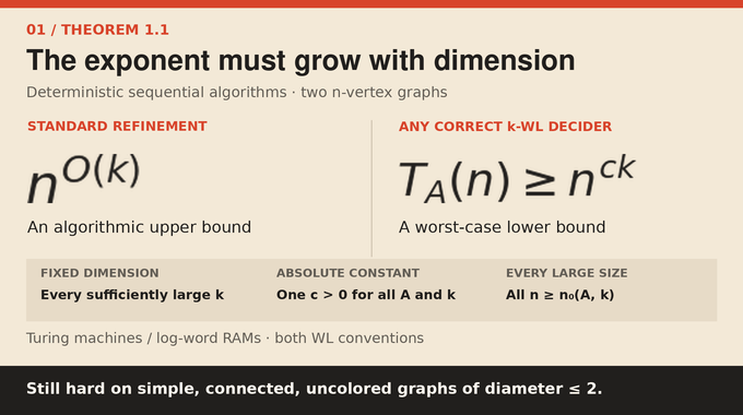
Here is algorithm ’s maximum time over permitted graph pairs of order , meaning vertices per graph. One absolute positive works for every sufficiently large fixed and every correct algorithm. The starting threshold may depend on both. Each size has a hard pair, rather than every pair being hard.
The models are multitape Turing machines and sequential RAMs with logarithmic-length words and addresses, bounded memory accesses per instruction, and fixed instructions computable in polynomial bit time. The fixed dimension WL complexity result covers both conventions. It does not assert an exact bound or measured practical slowdown. It rules out time without relying on the Exponential Time Hypothesis.
5. How Do Bijective Pebble Games Capture k-WL Equivalence?
Spoiler probes the graphs using paired markers. After discarding marked pairs, Spoiler requests a vacant pair. Duplicator must announce a vertex bijection before Spoiler selects a vertex. The selected vertex and its image receive the markers. Duplicator loses if marked vertices fail to preserve equality, adjacency, or colors.
The bijective pebble game in Lemma 2.3 characterizes stable equivalence: joint -WL needs pairs, while separate -WL needs pairs. The construction writes this budget as , with or , respectively. Its central maneuver uses pairs to expose an address and one spare pair to move information. A response chosen only after seeing Spoiler’s vertex would not meet the required game rule.
6. How Does the Proof Compress Addresses Into Blocks?
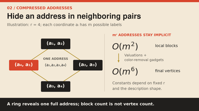
Imagine variables indexed by addresses with coordinates, each chosen from . Listing every address would destroy the reduction’s size advantage. Instead, site blocks store two neighboring coordinate labels in a cyclic row arrangement. Square blocks connect neighboring types through matched labels. Each block has only a bounded number of valuations for fixed parameters.
Values lie in vector spaces over , where addition is modulo two. Named vector or scalar readouts are shared between blocks. Vertices represent legal valuations, and edges join valuations in distinct blocks when all shared readouts agree. The construction compares homogeneous equations with an affine version containing prescribed offsets.
Individual-edge arc consistency asks for nonempty sets of vectors at each addressed variable whose scalar images match on each comparison separately. Supporting vectors may differ between comparisons. No single globally compatible assignment is required.
For a four-coordinate address, the four site blocks carry label pairs , , , and . Together they reveal the address. Summing their readouts cancels corner potentials and recovers its vector value. The spare pebble transports that value through square blocks along a subdivided wire.
Theorem 3.2’s compressed reduction enumerates blocks, with constants depending on fixed dimension and description shape. Removing colors attaches degree-distinguishing marks to valuation vertices, increasing the final count to . A universal hub guarantees diameter at most two. Confusing block count with final vertex count would invalidate the later exponent accounting.
A comparison concerns equality of two scalar-image sets. For example, an endpoint can offer several vectors producing the same scalar, and another comparison can use different supporting vectors from that same set. This flexibility is deliberate. Requiring one vector to satisfy every incident comparison would impose a stronger global condition than the reduction represents.
7. Why Are Wrapping Rings, Corner Potentials, and Exact Projection Essential?
The difficult direction constructs Duplicator’s strategy from consistency witnesses. Long subdivisions ensure that any collection of at most blocks has tree-shaped type support containing at most one original variable type. Thus a small query cannot impose arbitrary simultaneous requirements across distant variables.
A collection wraps when its corner graph has a closed walk crossing the distinguished cyclic seam an odd number of times. Lemma 3.5 shows that wrapping needs at least blocks. With exactly , it recovers a consistent full address. All such witnesses inside one permitted collection recover the same aligned address.
The proof assigns shifts to components and potentials to corners. Horizontal readouts combine their two corner potentials with a shift on the seam. Vertical readouts combine the relevant linear images of endpoint potentials. Around a full site ring, each potential occurs twice and cancels, exposing the shift.
Here is the family of compatible affine offset assignments for block collection , and the vertical bar means restriction to . Lemma 3.6 proves exact projection: every retained assignment extends, not merely some assignment.
On nonwrapping components, changing shifts can be absorbed into corner potentials without changing retained readouts. On wrapping components, matching scalar-image witnesses provide the required extension. Lemma 3.7 then translates each homogeneous block’s valuations by an offset. Duplicator independently chooses an extension for every prospective new block before announcing the combined bijection. Whichever vertex Spoiler selects, that block’s extension preserves the invariant, including nonadjacency.
The seam is the last cyclic row. Its shift contribution is recorded by a bit that is one there and zero elsewhere. Nonwrapping means these seam bits sum to zero along every closed walk. Path sums can then define consistent corner corrections, explaining why changing an unexposed shift leaves all old readouts intact.
8. How Can Symmetric Consistency Constraints Simulate Directed Computation?
Direct equality would transmit destination restrictions backward. Proposition 4.1 avoids this with a private buffer having two binary coordinates:
These equations denote three separate equalities of scalar images, rather than one simultaneous relation. If the source image is , both buffer coordinates must be zero, forcing destination image . For a source with image , the buffer can preserve both coordinate values while restricting their sum.
| Destination Image | Allowed Buffer Vectors | Each Coordinate Image |
|---|---|---|
In the first row, each buffer coordinate individually takes zero and one, although the sum is always zero. For source value one, the first comparison can use , and so can the second. Each comparison finds support separately. The destination therefore need not force the source image to collapse.
The circuit is monotone and acyclic. Scalar gates act as OR gates. Each two-port AND gate outputs the sum of its coordinates, with each port receiving an OR of incoming signals. Truth forces output image . A seed enforces zero, while a terminal test enforces one.
A true test therefore contradicts consistency. Conversely, when every test is false, explicit nonempty vector sets and these buffers satisfy every comparison. Terminality matters because a false test has image , rather than the full image used for ordinary false sources. This proves that consistency exists exactly when every test is false.
9. How Is a Turing-Machine Computation Encoded Into Two Graphs?
Theorem 4.3 divides the address digits into time and tape position. With , there are times and positions. Time does not wrap. Tape position is cyclic, but the stated space inequality prevents the visited region from colliding around the ring.
The exact capacity assumptions are and , where bounds halting time on every input of length . The first leaves enough time layers. The second makes reduction modulo the position-ring length injective on an interval containing the input and all relevant visited cells.
A fixed local rule updates each cell from its previous left, center, and right symbols, including head-state information. Two AND gates recognize each candidate triple, then feed the scalar gate for its resulting symbol. Induction shows that exactly the actual symbol is true at each time-position pair. Halting configurations remain frozen.
Incrementing base- digits is decomposed into carry cases with product domains. Decrement uses analogous borrow cases. This represents neighboring times and positions through short coordinate tables, rather than enumerating the full computation. The tables are generated from the input in time without running the encoded machine.
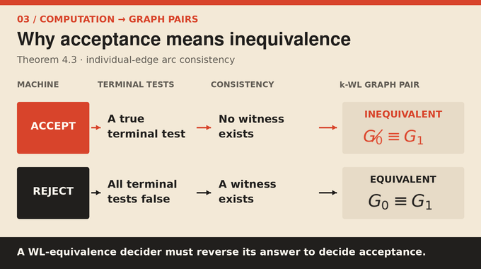
Terminal tests check accepting states at the last time. The computation reduction’s polarity is essential: acceptance creates a true test, destroys consistency, and produces graph inequivalence. Rejection leaves the graphs equivalent. This is a precise simulation, comparable in method to studying computation encoded in another mathematical system, rather than a claim that the reduction executes the long computation.
10. How Does Diagonalization Make the Time Lower Bound Unconditional?
Theorem 5.2 constructs a language for each positive integer . An input can begin with a self-delimiting machine description, followed by arbitrary padding. Membership reverses whether that designated machine accepts the entire input within steps, where is input length. Invalid designations are rejected.
Suppose a correct one-tape decider decides this language within that cutoff on an input beginning with its own description. If it accepts, the definition excludes the input. If it rejects, it has not accepted within the cutoff, so the definition includes it. Either answer contradicts correctness.
Padding makes such self-designating inputs available at every sufficiently large length. Consequently, every correct one-tape decider has worst-case time strictly greater than at each such length. This is stronger than hardness on an unspecified infinite subsequence.
The language remains decidable by a clocked universal simulation. The paper gives a one-tape upper bound , enough to fit its computation into the compressed reduction when dimension is large. The argument needs no unproved complexity separation. Its careful simulation accounting connects naturally with time and space bounds for Turing machines.
11. Why Does the Proof Hold at Every Large Graph Size, and What Remains Unproved?
For input length , pad the graph pair to every integer size in . Constructing its explicit matrices costs time. A fixed auxiliary decider tries every size in this interval, simulating the candidate WL algorithm up to a cutoff on each trial. If none completes, it falls back to the diagonal language’s known decider.
One size with a sufficiently fast worst-case graph algorithm would make that trial finish for every word of length . Reversing its answer would decide the diagonal language too quickly. The simulation overhead has an absolute polynomial exponent, allowing the proof’s parameter choices to force the contradiction.
The cutoff exponent is chosen much smaller than the diagonal exponent , both growing with . The one-tape trial procedure takes at most time for an absolute constant . Choosing and makes the graph-time assumption contradict the language bound.
These intervals cover every sufficiently large integer size. Trying all sizes eliminates isolated fast orders without assuming runtime is monotone. That is the final step from compressed computation to the eventual k-WL time lower bound.
The result remains asymptotic and model-specific. It supplies neither an optimal exponent constant nor practical runtime measurements. It does not prove randomized or nonuniform lower bounds, a bounded-degree promise, or a comparable graph-isomorphism lower bound. The hub has unbounded degree. Small dimensions require a separate unrestricted input-reading observation. As with query complexity and algebraic complexity, the computational model determines what the conclusion means.
The supplied Lean scope document for family 133 explicitly includes the unconditional theorem, both refinement conventions, and the diameter-two promise. This article checks the paper and scope statement, rather than independently rebuilding the formalization.
The central lesson of weisfeiler leman time complexity is that bypassing refinement cannot remove dimension’s linear contribution to the exponent under these assumptions. Follow Binary Verse AI’s mathematical proof coverage for explanations that connect formal statements to the mechanisms that make them work.
What is the time complexity of the Weisfeiler–Leman algorithm?
For fixed dimension , straightforward algorithms for k-dimensional Weisfeiler–Leman equivalence run in time. OpenAI proves that every correct deterministic sequential decider in the specified models requires worst-case time for sufficiently large fixed . Thus an exponent growing linearly with is unavoidable up to constant factors in the exponent.
Does OpenAI’s proof establish an exact lower bound?
No. The theorem establishes for an absolute positive constant , not necessarily . It rules out algorithms with running time , but it does not establish the optimal constant multiplying in the exponent.
Why is the Weisfeiler–Leman lower bound unconditional?
The proof does not assume ETH, P ≠ NP, or another unproved complexity separation. It constructs an explicitly hard language through diagonalization, reduces its computation to graph equivalence, and derives a contradiction from the existence of an excessively fast deterministic decider.
Does the lower bound apply to 1-WL, 2-WL, and 3-WL?
The main theorem establishes its strong bound for every sufficiently large fixed . It does not give the same promised-class result individually for small dimensions. The paper separately discusses input-reading lower bounds for smaller on unrestricted adjacency-matrix graphs.
How do joint and separate Weisfeiler–Leman refinement differ?
Joint refinement records the multiset of complete coordinate-replacement color vectors. Separate refinement records an independent replacement-color multiset for each coordinate. Their game characterizations consequently differ: joint -WL corresponds to pebble pairs, whereas separate -WL corresponds to pairs. The paper proves lower bounds for both conventions.
Why does the proof work even for connected graphs of diameter two?
The construction removes vertex colors through degree-distinguishing gadgets and adds a universal hub, making the resulting graphs connected with diameter at most two. These transformations preserve the relevant equivalence. This shows the hardness is not merely caused by disconnected or long-diameter graph structures.
Does this result prove that graph isomorphism cannot be solved faster?
No. Graph isomorphism and k-WL equivalence are different decision problems. The theorem establishes a worst-case lower bound for deciding whether two graphs have the same stable k-WL color histograms. It does not establish a comparable lower bound for arbitrary graph-isomorphism algorithms.