
Remove the alternating signs from a determinant, and a familiar matrix formula becomes a central challenge in algebraic complexity. OpenAI’s September 24, 2026 paper advances the permanent vs determinant problem by proving a cubic lower bound on the size of determinant representations, even when coefficientwise limits are allowed. The previous unrestricted complex border bound was quadratic. The result concerns representation size, not a cubic running-time requirement, and the superpolynomial conjecture remains open.
The research manuscript builds its argument around a specially extracted coefficient, geometry in characteristic two, and a count of polar intersections. Those ingredients explain how the exponent changes. OpenAI released the work within its October mathematics collection; the proof’s mathematical content deserves closer attention than the announcement’s scale.
Table of Contents
1. Permanent vs Determinant Problem: Why Does One Sign Matter?
For a square matrix, both polynomials sum products that select one entry from every row and column. The determinant attaches a sign according to permutation parity. The permanent omits that sign. For a two-by-two matrix, the distinction is:
In a bipartite graph, rows and columns represent the two vertex classes, and entries represent edge weights. Each perfect matching contributes its weight product to the permanent. With zero-or-one entries, the result counts perfect matchings. With arbitrary weights, including negative ones, it is a weighted sum.
The question is whether a larger determinant can reproduce this polynomial after substituting affine-linear expressions into its entries. Simply noticing the sign difference does not settle how large that determinant must become.
For example, setting all four entries to one gives determinant zero and permanent two. The cancellation is visible immediately. At larger orders, however, a clever representation can introduce extra rows, columns, and constants. A lower bound must defeat every permitted encoding, rather than just compare the two original matrices.
| Topic | Paper’s Statement |
|---|---|
| Research Object | Permanent of an matrix |
| Main Advance | Cubic lower bound on complex border determinant size |
| Explicit Estimate | for |
| Allowed Representations | Arbitrary affine-linear entries and coefficientwise limits at fixed order |
| Still Open | Superpolynomial determinant size; broader complexity separations |
2. What Are Determinantal Complexity and Border Determinantal Complexity?
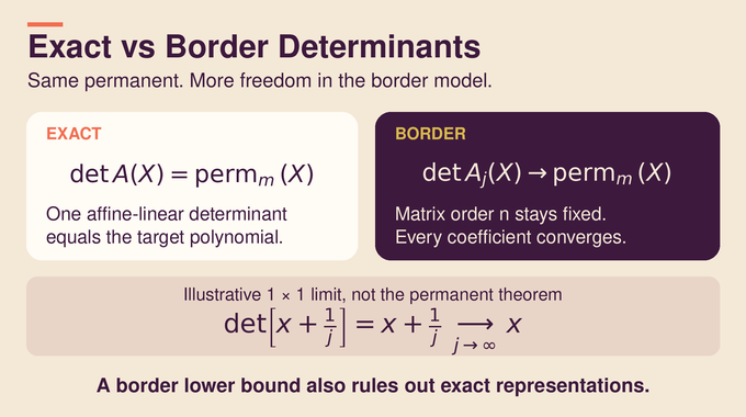
Determinantal complexity, written , is the smallest positive matrix order permitting:
Here counts input variables, and each is a constant complex matrix. Every entry may mix all variables plus a constant. This is more permissive than substituting only individual variables or constants.
Border determinantal complexity, denoted , also allows coefficientwise limits. Fix the matrix order, form a sequence of determinant polynomials, and require every monomial coefficient to converge to its coefficient in . Matrix-entry coefficients themselves need not stay bounded.
This is not numerical approximation at selected inputs. It is convergence of whole polynomials in a finite-dimensional coefficient space. Exact representations are constant sequences, so border complexity cannot exceed exact complexity. Proving a border lower bound therefore rules out more possible shortcuts.
The fixed-order requirement matters. Allowing the determinant size to increase along the sequence would change the question. Here the approximating expressions can become badly conditioned or use enormous coefficients, but they cannot quietly purchase extra matrix dimensions while approaching their target.
As with exact-arithmetic Fourier complexity, the allowed operations and coefficients determine what the theorem actually says.
3. The Quadratic Barrier: Why Earlier Proofs Could Not Go Further
Mignon and Ressayre obtained the characteristic-zero exact bound . Their tool was the Hessian, the matrix of second partial derivatives. At a suitable permanent zero its rank is , while an order- determinant at a singular matrix has Hessian rank at most . Affine substitution cannot increase that rank.
Landsberg, Manivel and Ressayre established the same quadratic scale for unrestricted complex border representations through projective geometry involving degenerate dual hypersurfaces. The new paper improves the exponent in that model.
“Barrier” here describes the reach of previous bounds, not a theorem forbidding every refinement of earlier methods. Another obstruction, based on the singular locus, is too small for the permanent itself: matrices with two zero columns give a singular family of codimension at most .
The paper therefore changes the object under examination. Instead of squeezing harder on the permanent’s existing singularities, it extracts a related polynomial and finds a smooth restriction with many variables. That construction creates geometry that a different lower-bound argument can exploit.
4. OpenAI’s Cubic Lower Bound: What Does the Theorem Actually Prove?
Theorem 1.1 states the following explicit permanent determinant lower bound over the complex numbers:
The symbol is the base of natural logarithms. The authors do not optimize the constant. The headline is asymptotic cubic growth, written , rather than a useful threshold for small matrices. Indeed, this conservative explicit estimate need not beat the older quadratic numerical bound near its starting threshold.
No symmetry condition restricts the determinant pencil. The theorem permits arbitrary complex affine-linear entries and arbitrary coefficientwise limiting sequences at a fixed order. It also transfers to exact determinantal complexity.
The manuscript is a preprint with a published formalization scope. This article explains its theorem and argument; it does not report an independent Lean rebuild or completed journal review. As our AI mathematical proofs analysis emphasizes, improving a bound and resolving its parent conjecture are distinct achievements.
5. Constructing the Coefficient Polynomial That Unlocks the Proof
Introduce an auxiliary matrix size , a diagonal parameter matrix , and two bookkeeping variables . Define:
The brackets select one coefficient. Choosing diagonal contributions from and another from leaves exactly factors from . Thus is homogeneous of degree in the matrix entries.
The two selected diagonal sets must be disjoint. Once they are removed, the surviving terms form the permanent of the complementary principal submatrix, weighted by the selected diagonal parameters. No additional factorial appears in this coefficient expansion.
This degree-and-variable balance is deliberate: degree grows linearly with , while the available variables grow quadratically. The coefficients are integral polynomials in the parameters, allowing the same definition to be specialized into different characteristics. The proof will use that portability without assuming that every accompanying construction survives the journey.
6. Count Gates and Cancellation Gadgets: Encoding the Coefficient as a Permanent
Coefficient extraction is not automatically a cheap permanent substitution. The paper constructs two counting gates, one for each selected diagonal type, enforcing exactly choices per type.
Each gate contains original rows and columns plus additional rows and columns. Once the chosen distinguished edges are fixed, the remaining cross-matchings have completions. Both gates together contribute the fourth power of that factorial.
A signed equality gadget couples each special main edge to its gate edge. It adds three internal rows and columns. Summed internal completions cancel unless both paired edges are used or both are unused. Their respective weights are and , where is the main edge’s weight. Cancellation enforces agreement without inspecting individual matchings.
There are gadgets. Counting the main matrix, gates, and internal blocks gives permanent order . The output equals times the nonzero complex scalar . Rescaling one row removes it. Identity padding permits any larger order.
Crucially, that scalar vanishes in characteristic two. The next stage uses the integral coefficient formula directly, not a reduction of this scaled graph identity.
7. Why Characteristic Two Makes the Adjugate Construction Possible
Work over an algebraic closure of the two-element field, not merely its two elements, so arbitrarily many distinct parameters are available. Since positive and negative signs coincide, permanent equals determinant. With distinct diagonal parameters, each matrix determines the projective plane curve:
The extra coordinate homogenizes the expression. On the line , the determinant splits into distinct factors . This fixed boundary makes the curve reduced and its projection to finite and generically separable.
The adjugate, the transposed cofactor matrix, defines a finite subscheme on this curve. A scheme records multiplicity as well as point locations. If every entrywise derivative of vanishes, the coefficient vanishes in every adjugate entry.
The paper proves those entries span all degree- forms vanishing on . Complementary monomials then show no nonzero degree- form vanishes there, using . Consequently , where , the dimension of degree- plane forms.
The complementary-monomial step is a coefficient detector. Multiply a chosen monomial’s contribution by the powers needed to reach the selected coefficient. Exactly that contribution survives extraction. If a degree- form vanished on the scheme, every one of its coefficients would therefore vanish. The length bound counts independent information, including nonreduced multiplicities.
8. Conductor Ideals and Normalization Defects: Bounding the Critical Locus
Normalization separates the local branches of a reduced curve into a nonsingular model. Its defect measures the length of the missing local functions, accounting for singularities and intersections between components.
The conductor ideal consists of curve functions that still belong to the original curve ring after multiplication by any normalized function. The paper shows this ideal lies inside the adjugate ideal. A colength identity then yields . Every critical matrix therefore produces a curve with defect at least .
An arbitrary-characteristic Severi dimension theorem bounds the family of such curves by . But curves alone do not count matrices: several matrices can determine the same curve.
To control these fibers, the proof sums the adjugate rows. Its zero subscheme has length , and the fixed boundary frame makes that subscheme determine the matrix uniquely. A Hilbert-scheme estimate bounds the matrix fiber by the same length. Adding the two dimensions gives a critical-locus dimension at most , hence codimension at least .
This is the geometric payoff: vanished derivatives force enough curve defect that critical matrices occupy a comparatively small part of matrix space.
Both dimension estimates are essential. A rare family of curves could still conceal a large family of representing matrices if its fibers were uncontrolled. The adjugate-row construction closes that gap. The full adjugate measures defect, while its row-sum subscheme provides the separate information needed to distinguish matrices over one curve.
9. Returning to Complex Numbers: Constructing a Smooth Hypersurface
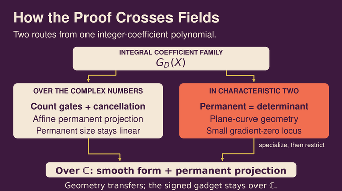
Moving from characteristic two to complex numbers requires more than reinterpreting symbols. The integral parameter family defines the projective zero scheme of its raw partial derivatives. Projectivity makes the family proper, so upper semicontinuity of fiber dimension carries the small-gradient-locus bound to an open neighborhood of the characteristic-two parameter point.
The parameter base is integral. That nonempty open neighborhood contains its characteristic-zero generic point and has complex points. This supplies suitable complex parameters without lifting individual characteristic-two matrices.
Only now does Euler’s homogeneous identity identify gradient zeros with hypersurface singularities: the positive degree is invertible over the complex numbers. The argument deliberately avoids that division during characteristic-two specialization.
For , choose . The codimension estimate lets a general -dimensional linear subspace avoid the singular scheme and meet the smooth locus transversely. Restricting gives a nonzero smooth projective hypersurface of degree .
The earlier complex gadget construction now applies at these parameters. After rescaling, the restricted polynomial is an affine restriction of a permanent of order at least . The two branches of the proof have finally met.
Smoothness here means every projective zero has a nonzero differential. It does not require the original coefficient polynomial to be smooth everywhere. Selecting a suitable linear subspace removes its problematic directions while preserving the degree and enough variables for the final count. Avoiding singular points alone would be insufficient without the additional transversality condition.
10. Polar Intersections and Kernel Equations: The New Lower-Bound Argument
A first polar is a directional derivative. For the smooth degree- hypersurface in projective dimension , choosing general polars gives exactly distinct simple intersection points. “Simple” means the local equation system has invertible Jacobian.
These selected points persist for one sufficiently close determinant approximation, by the complex implicit function theorem. Only polynomial coefficients must be close. The approximating matrix entries may be arbitrarily large.
At each surviving point the determinant matrix has rank exactly . Introduce its right and left kernel lines, represented by . The determinant and polar conditions become bilinear equations involving the input coordinates, , and , including , where differentiates the matrix in the chosen direction.
A local Schur-complement argument proves the lifted solutions remain simple. A multihomogeneous count bounds these selected solutions even if other components exist. The comparison is:
Taking roots yields . The decisive gain is a product of degree and variable count. Smoothness supplies a large finite certificate; kernel equations limit how many certificate points a small determinant can support.
This persistence step is what makes the argument a border proof. Counting only the target’s geometry would leave open the possibility that nearby determinants behave differently. Tracking finitely many simple solutions into one actual approximant supplies a common object on which the lower and upper counts can be compared.
11. From the Quadratic Barrier to a Cubic Bound: Completing the Proof
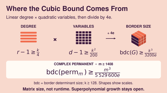
Set . For , the construction applies, and its estimates give:
The first inequality follows because fixed affine substitution cannot increase border determinantal complexity. Linear degree and quadratic variable count produce the cubic exponent.
| Model | Lower Bound | Qualification |
|---|---|---|
| Border Determinants | matrix order | Arbitrary complex affine-linear coefficientwise limits |
| Exact Determinants | Same explicit cubic estimate | Included as constant approximating sequences |
| Branching Programs | vertices and edges | Affine labels; limits retain fixed vertex or edge budgets |
An algebraic branching program sums products of affine edge labels along source-to-sink paths in a directed acyclic graph. A program with vertices yields a determinant of order ; after trimming, edges yield order at most . Thus the algebraic branching program lower bound is cubic, including limits with fixed vertex or edge budgets.
The published Lean scope covers the exact and border permanent bounds and a supporting smooth-initial-form theorem. It excludes those branching-program consequences. Our Lean formalization explainer discusses why matching formal statements to headline claims matters.
Valiant’s conjecture, VP versus VNP, and P versus NP remain unresolved by this result. Developers gain no runtime benchmark or implementation speedup. Researchers gain a geometric obstruction that survives unrestricted determinant limits. The permanent vs determinant problem remains open, with a stronger lower bound and a proof strategy to investigate. Follow Binary Verse AI’s AI and mathematics coverage for explanations that connect the theorem, its proof, and its remaining questions.
What is the difference between the permanent and determinant of a matrix?
Both sum products indexed by permutations. The determinant assigns a positive or negative sign according to permutation parity; the permanent omits that sign. For a two-by-two matrix with rows (a, b) and (c, d), the determinant is ad − bc and the permanent is ad + bc. This sign difference is central to the representation problem.
What is the permanent vs determinant problem?
It asks how large a matrix of affine-linear forms must be for its determinant to equal the permanent of an m-by-m matrix. The central unresolved question is whether the required determinant size must grow superpolynomially. The cubic lower bound advances this question without settling it.
What is border determinantal complexity?
Border determinantal complexity is the minimum determinant size when coefficientwise limits of affine-linear determinant representations are allowed. The size stays fixed along the approximating sequence, although matrix-entry coefficients may be unbounded. The paper proves that even these limiting complex representations require asymptotically cubic matrix order.
How did OpenAI’s proof overcome the previous quadratic lower bound?
The proof constructs a smooth homogeneous polynomial as an affine restriction of a permanent. Characteristic-two plane-curve geometry bounds the coefficient polynomial’s critical locus, and specialization supplies suitable complex parameters. Polar-intersection counting then gives a lower bound proportional to degree times number of variables, producing cubic growth.
Why does the proof use characteristic two if the result concerns complex numbers?
In characteristic two, the permanent and determinant coincide, enabling the adjugate and plane-curve construction. The integral coefficient polynomial defines a proper family of projective gradient-zero schemes. Upper semicontinuity transfers the dimension bound to suitable complex parameters. The graph projection’s scaling factor vanishes in characteristic two, so that projection is used only over the complex numbers.
Does the cubic lower bound solve Valiant’s conjecture or P versus NP?
No. It strengthens a quadratic lower bound to cubic growth for determinant representations, but does not establish superpolynomial determinantal complexity, separate VP from VNP, or resolve P versus NP. It is also not a cubic running-time lower bound for computing the permanent.
Has OpenAI’s permanent–determinant proof been formalized in Lean?
OpenAI’s published Lean scope documentation reports formalizations of the cubic exact and border determinant lower bounds and a supporting smooth-initial-form theorem. The paper’s algebraic-branching-program consequences are outside that stated scope. This article does not report an independent rebuild of the Lean development.