
A convex body can become smaller when you replace arithmetic averages with geometric ones. The logarithmic Brunn Minkowski conjecture asks whether its volume nevertheless stays above a precise lower bound. OpenAI’s paper proves that it does for any two origin-symmetric convex bodies, in every dimension. The result rests on a sharp variance inequality, a transport construction, and a tensor calculation that turns an uncertain sign into explicit squares. Here is how those pieces connect, why symmetry matters, and exactly what follows for volume and log-concave measures.
Table of Contents
1. What OpenAI Proved About the Logarithmic Brunn–Minkowski Conjecture
Theorem 1.1 states the result for convex bodies , with , satisfying and . For :
Here means ordinary -dimensional volume, is the support function, and constructs a convex body from directional bounds. Origin symmetry means reflection through zero leaves the body unchanged. A convex body is compact, convex, and has nonempty interior.
| Item | Verified Statement |
|---|---|
| Objects | Full-dimensional origin-symmetric convex bodies. |
| Dimensions | Every . |
| Interpolation | Geometric means of support bounds, followed by Wulff intersection. |
| Proof engine | Sharp variance bound in moment coordinates. |
| Consequences | Symmetric inequalities and scalar (B)-concavity. |
The September 23, 2026 paper supplies a mathematical proof. OpenAI’s release announcement describes Lean formalizations for many released results, but does not establish this particular proof’s formalization scope. Our guide to OpenAI’s mathematical proofs provides broader context. The theorem itself requires no computational benchmark.
2. The Original Problem: Classical vs Logarithmic Brunn–Minkowski Inequality
Minkowski addition combines every point of one set with every point of another. Its weighted version contains points , where and . The classical Brunn Minkowski inequality says that the volume’s th root is concave under this interpolation:
The arithmetic–geometric mean inequality then gives the weaker multiplicative lower bound used in the logarithmic theorem. Crucially, the logarithmic Wulff body sits inside the ordinary Minkowski combination. Proving that this potentially smaller body still achieves the geometric-mean volume bound is a strengthening of the classical multiplicative statement.
Arithmetic interpolation averages directional support distances. Logarithmic interpolation averages their logarithms, equivalently taking geometric means of positive distances. The conjecture concerns this different operation on shapes. It does not merely insert logarithms into the classical formula. The endpoints recover the original bodies, so equality there is automatic.
3. Why the Higher-Dimensional Conjecture Was Difficult
The paper credits Böröczky, Lutwak, Yang, and Zhang with the planar proof. Earlier results also covered unconditional bodies sharing a coordinate basis, bodies with suitable common reflection symmetries, and complex norm balls. Unconditional means invariance under every coordinate sign change. Such assumptions organize the geometry enough to support specialized arguments.
Local approaches studied second variations of volume. Kolesnikov and Milman expressed the issue through an even spectral inequality for the Hilbert–Brunn–Minkowski operator. Other work obtained parameters close to the classical case, or local logarithmic results for zonoids, which are limits of sums of segments. These advances did not directly settle arbitrary symmetric pairs at the logarithmic endpoint.
The analytic difficulty was controlling the required second variation without extra geometric structure. OpenAI’s paper also acknowledges Stancu’s earlier all-dimensional announcement, whose report deferred flow-asymptotic details. It presents a separate proof through a summandwise variance estimate. Historical credit therefore includes both established special cases and that earlier announcement, without conflating their proof mechanisms.
4. Support Functions and Wulff Bodies: Defining the Logarithmic Sum
For a unit direction , the support value is . The inner product measures distance along that direction. Symmetry and nonempty interior ensure positive support values. For a positive continuous function on the unit sphere:
The sphere contains all unit directions. Each inequality defines a supporting half-space. Intersecting them gives the Wulff body. The geometric mean of support functions can fail to be a support function, so this intersection cannot be omitted.
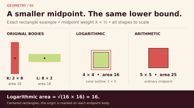
Consider centered rectangles with half-widths and , using . Their logarithmic interpolation is exactly the square with half-widths . Indeed, for nonnegative , . This verifies every directional constraint, while coordinate directions bound the result inside that square.
| Body | Half-Widths | Area |
|---|---|---|
| 16 | ||
| 16 | ||
| Logarithmic Wulff body | 16 | |
| Arithmetic Minkowski body | 25 |
This is exact geometry, not a schematic.
The example shows why the strengthening has content even for familiar shapes. Both endpoints have area sixteen, and the logarithmic midpoint attains the required lower bound exactly. The arithmetic midpoint has larger area because it retains more width in both coordinate directions. Equality here does not mean that the two original rectangles are identical. It also cautions against assuming that every equality case must consist of scalar copies of one body. The paper’s main theorem states the inequality without providing a complete new classification of all equality cases. For a different question about convex representations, see our generalized Lax conjecture explainer.
5. The First Reduction: Replacing Convex Bodies With Finite Slab Intersections
Instead of handling infinitely many directions immediately, choose finitely many spanning vectors and positive widths . Each constraint defines a symmetric slab between parallel hyperplanes. Their intersection is a bounded symmetric polytope. Spanning prevents an unbounded direction, while positive widths leave an interior neighborhood of zero.
Interpolate each width geometrically between its endpoint values:
The first target is log-concavity of the polytope’s volume along this path. The intermediate polytope need not share an unchanged face structure with its endpoints. Its defining inequalities still make sense when some constraints become redundant.
Later, nested finite direction sets, containing coordinate directions and with dense union on the sphere, recover every supporting inequality. This gives a manageable finite problem without imposing a common normal fan on the original bodies. The passage back to arbitrary shapes uses continuity rather than an assumption that every body is already polyhedral.
6. Smooth Approximation: Turning Hard Geometric Constraints Into Integrals
A sharp indicator switches abruptly at the polytope boundary. Replace it by a smooth exponential weight. For an even integer and , set:
Define . Each even power is nonnegative and convex. Inside a slab it tends to zero as the power increases, while outside it diverges. The exponential weight consequently approaches the slab intersection’s indicator, multiplied by the Gaussian regularizer, away from boundary hyperplanes.
The Gaussian term ensures integrability and , meaning uniform convexity. It also dominates differentiated integrands by an integrable Gaussian times a polynomial. This justifies differentiating under the integral when the widths vary. Smoothing supplies both calculus and the transport hypotheses needed later. It is an intermediate proof device, not a claim that Gaussian-weighted volume equals ordinary volume before taking limits.
7. The Key Insight: A Variance Inequality Controls Volume
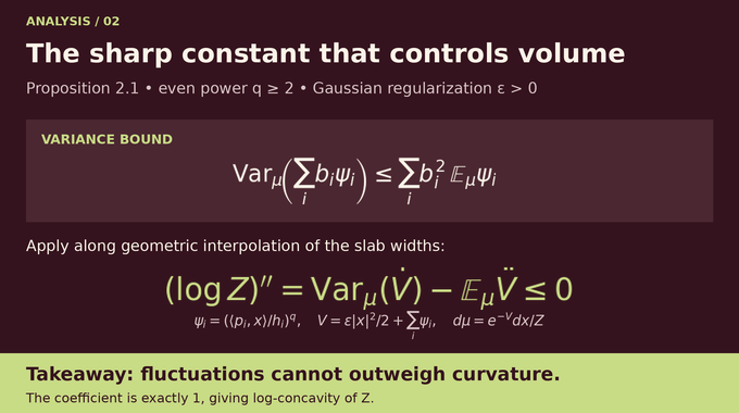
Normalize the smooth weight to a probability measure . Expectation averages under that measure, and variance measures squared deviation from the mean. Proposition 2.1 states, for arbitrary real coefficients :
The constant is exactly one. This matters because geometric width interpolation gives , hence and . Dots denote derivatives with respect to . Differentiating the normalizing integral yields:
The variance bound makes the fluctuation term no larger than the expected curvature term. Therefore the smooth integral is log-concave along the interpolation. This is the bridge from an analytic inequality to the geometric theorem.
No independence assumption separates the slab potentials. They are functions of the same point and may have substantial correlations, especially when directions are redundant or nearly aligned. The proposition controls every real linear combination despite that dependence. An estimate with a larger constant would not supply the displayed concavity conclusion by this argument, because the second derivative term has a fixed coefficient. This explains why a familiar qualitative concentration statement would be insufficient.
Log-concavity also appears in log-concave sampling, but this proof establishes a volume inequality rather than a runtime guarantee for a sampler.
8. Moment Coordinates: Constructing the Transport Behind the Proof
The proof changes coordinates using a smooth even convex potential . Its gradient map transports the probability measure to . Transport means that averaging a function of under equals averaging its composition with this gradient under .
The Jacobian is the Hessian . Conservation of probability gives the Monge–Ampère identity:
Lemma 3.1 constructs a global smooth diffeomorphism and proves . Positive definiteness holds everywhere, but no uniform positive lower bound is asserted across the whole space. That distinction matters for the later cutoff arguments.
The construction combines compact moment results, Klartag’s moment-Hessian estimate, and a smooth limiting argument. It verifies that the gradient reaches the entire target space. The coordinates are useful because their Hessian supplies an integration-by-parts structure adapted to the target probability, rather than merely relabeling points.
9. Adjoints and Even Test Functions: Removing the Spectral Obstruction
Write , evaluated at the corresponding target point. Define negative weighted divergence by . The associated operator is:
The colon means matrix contraction. For a compactly supported smooth even test , construct , , and . On matrices, divergence acts row by row. Two integrations by parts express through either the gradient or the Hessian of .
Lemma 5.1 proves these double-divergence tests are dense among centered even square-integrable functions. Centered means zero expectation, and even means unchanged by .
Why those restrictions? Constants satisfy , while coordinate functions satisfy . Thus annihilates affine functions. The lemma proves there are no additional obstructions. Centering removes constants and evenness removes linear functions. Its cutoff proof uses the global upper Hessian bound together with local positivity, avoiding an unjustified global lower bound.
10. The Decisive Tensor Estimate: Why the Variance Bound Holds
Lemma 6.1 controls two nonnegative energies using . With and , it bounds their sum:
A weighted Bochner identity first splits into a Hessian energy and a derivative-trace term. The latter is a matrix-square trace, not automatically a Euclidean squared norm for an arbitrary vector field. The moment-coordinate structure supplies the needed sign through a separate calculation.
After a constant coordinate normalization, the remaining tensor expression becomes , plus another nonnegative square. Here records third derivatives of the test, couples its Hessian to third derivatives of , and swaps its first two indices.
Homogeneity then gives . Two Cauchy–Schwarz estimates, using the gradient and Hessian pairings separately, produce complementary contributions. Together they yield . Density extends this dual estimate to all centered even tests. One final Cauchy–Schwarz application proves Proposition 2.1. The paper relates this framework to earlier Brascamp–Lieb and transport-Hessian work.
11. Completing OpenAI’s Proof in Every Dimension
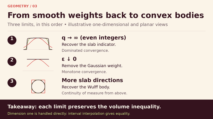
The remaining steps return from analysis to geometry. First, Proposition 2.1 proves log-concavity of the smooth integral for every fixed regularization and even power. Next let tend to infinity through even integers. Dominated convergence produces Gaussian-weighted volumes of the finite slab intersections. Their boundary hyperplanes have zero Lebesgue measure.
Then let . Monotone convergence removes the Gaussian factor and recovers ordinary polytope volumes. Finally increase the finite direction sets. The resulting bodies decrease inside a common bounded body, and continuity in the direction identifies their intersection with the desired Wulff body. Continuity of measure from above transfers the inequality to that limit.
The order of these arguments matters: each stage has its own domination, monotonicity, or boundedness justification. No exchange of unrelated limits is needed.
Dimension one is separate and elementary. For and , the interpolated interval has radius , giving equality in the volume bound. Combined with the higher-dimensional argument, this completes the stated every-dimension result.
12. Mathematical Consequences and the Exact Scope of the Proof
Corollary 1.2 establishes the symmetric Lp Brunn Minkowski inequality throughout . Its Wulff bound is , and the resulting volume raised to is at least . The argument normalizes endpoint volumes and reweights the interpolation parameter.
For measures, Saroglou’s transfer theorem extends the logarithmic inequality to even log-concave densities. The paper adds a support-subspace reduction for even log-concave Radon measures. These measures need only be finite on compact sets, not probability measures. Applying the result to scalar dilates proves log-concavity of , the scalar-dilation (B)-conjecture.
For a probability measure, this describes how the mass captured by an expanding symmetric body changes when scale is measured logarithmically. The body may be arbitrary within the stated hypotheses, but the same scalar multiplies every coordinate. That restriction is part of the consequence being proved, not merely a choice made for illustration.
The logarithmic Brunn Minkowski conjecture is therefore resolved within its origin-symmetric scope. This does not assert the unrestricted nonsymmetric inequality, general anisotropic dilation concavity, or an algorithmic speedup. Like our entropy photon-number inequality explainer, the useful takeaway is the exact inequality and its hypotheses. Follow Binary Verse AI for paper-led explanations that make the argument, assumptions, and consequences readable together.
What is the logarithmic Brunn–Minkowski conjecture?
It asks whether logarithmic interpolation between two origin-symmetric convex bodies produces a body whose volume is at least the weighted geometric mean of their volumes.
Did OpenAI prove the logarithmic Brunn–Minkowski conjecture in every dimension?
Yes. OpenAI’s September 23, 2026 paper proves the inequality for arbitrary origin-symmetric convex bodies in every dimension. The symmetry requirement is essential to the theorem’s stated scope.
Why is the logarithmic inequality stronger than the classical Brunn–Minkowski inequality?
The logarithmic Wulff interpolation lies inside the corresponding ordinary Minkowski combination. Establishing the same geometric-mean volume lower bound for this potentially smaller body is stronger than the classical multiplicative statement.
Why does OpenAI’s proof use a Wulff body?
The geometric mean of two support functions need not be a support function itself. The Wulff construction produces the correct convex body by intersecting the associated supporting half-spaces.
What is the main new mathematical argument in OpenAI’s proof?
A sharp variance estimate for sums of even powers of linear forms. Moment coordinates, a density theorem for centered even tests, and a tensor sum-of-squares calculation establish the estimate.
How does the proof extend from smooth approximations to arbitrary convex bodies?
It first lets the even exponent tend to infinity, then lets decrease to zero to remove Gaussian regularization. Increasingly dense sets of slab directions then recover the desired Wulff body and its volume.
Does OpenAI’s proof also establish the inequality and the (B)-conjecture?
Yes. It implies the symmetric Brunn–Minkowski inequality for every , along with the scalar-dilation (B)-conjecture for every even log-concave Radon measure and every origin-symmetric convex body.