
A sampler can know the exact slope of a probability landscape and still spend a dimension-dependent number of queries finding its way around. OpenAI’s manuscript changes that theoretical picture. For log concave sampling with a known minimizer and tightly bounded curvature, it proves that every fixed positive power of dimension can be avoided in the exact value-and-gradient query budget. The output is within total-variation distance one-tenth of the target distribution.
The qualification matters: computation between queries is unrestricted. This is a theorem about information access, not a demonstrated speedup for a Bayesian inference package. Its achievement is a finite construction that obtains high-order accuracy from a potential with only two continuous derivatives, then removes the Gaussian noise used to make that construction work.
Table of Contents
1. What Is Log-Concave Sampling, and Why Is It Difficult?
Sampling asks for random points with the right probabilities, rather than the single point that minimizes an objective. Here the target is a Gibbs distribution:
The potential assigns an energy to each point. The normalizing constant makes probabilities sum to one. Convexity of makes the log-density concave. For , the target is a standard Gaussian, with independent unit-variance coordinates.
| Research Artifact | OpenAI manuscript dated September 26, 2026. |
|---|---|
| Input Class | Twice continuously differentiable potentials on with a supplied minimizer and Hessian between identity and twice identity. |
| Oracle Access | An exact potential value and gradient at each queried point. |
| Output Accuracy | Total-variation distance at most from the original target. |
| Upper Guarantee | For every fixed , at most queries on every execution. |
| Lower Guarantee | At least queries for all sufficiently large dimensions. |
| Resource Limitation | Arithmetic, bit costs, and memory are not bounded by this query theorem. |
Even with one basin and no competing modes, most probability mass occupies a broad region rather than the minimizer. Sampling must reproduce that spread across many coordinates. Finding the bottom of the landscape does not finish the job. The switch-chain mixing problem illustrates the same distinction between producing a valid object and producing the correct distribution, in a discrete setting.
2. The Well-Conditioned Sampling Problem and Its Mathematical Assumptions
The manuscript normalizes the known minimizer to the origin and fixes the curvature window:
Here is dimension, is the identity matrix, and the matrix inequalities hold everywhere. Every directional curvature lies between one and two. This is strongly log concave sampling with fixed condition number, not arbitrary log-concave sampling with flat directions, constraints, or unknown conditioning.
An exact query returns both and . Query points may depend on previous replies and private randomness. The target accuracy uses total variation, the largest difference in probability assigned to any measurable event. Error one-tenth is a distributional discrepancy, not a ten-percent chance that a point is invalid.
A Gaussian prior combined with a suitable convex negative log-likelihood can motivate this kind of target, but an application must actually satisfy the theorem’s global curvature bounds. A locally well-behaved posterior is insufficient. Nonconvex neural-network posteriors are not covered simply because their inference code uses gradients. The known minimizer is another supplied resource, rather than a free preprocessing result.
Define as the smallest worst-case query cap achieving that accuracy for every permitted potential. The cap holds on every execution, rather than merely in expectation. These modeling choices are part of the theorem, not implementation details to discard later.
The accuracy is deliberately fixed throughout the main statement. It should not be read as a theorem with uniform constants for arbitrarily demanding error tolerances. Similarly, exact replies can carry information unavailable from finite precision evaluations. Translating this oracle result into numerical software would require a separate analysis of how rounding and approximate gradients propagate through the construction.
3. Why Previous Sampling Algorithms Faced a Polynomial Query Barrier
Langevin and Hamiltonian methods approximate continuous dynamics using discrete steps. Errors that look harmless in one coordinate can accumulate with dimension. Better discretizations reduce that dependence, but a positive dimension exponent remained in relevant guarantees under comparable curvature assumptions.
| Earlier Fixed-Parameter Routes | The manuscript cites bounds yielding fixed total-variation accuracy, including shifted-composition and diffusion-path approaches. |
|---|---|
| Smoothed Picard Result | A cited expected-gradient bound at fixed relative entropy converts to fixed total variation. Capping its budget preserves that exponent. |
| High-Accuracy Results | Separate bounds have different inverse-accuracy dependence. The manuscript discusses and subsequent results in that context. |
| Present Construction | Every fixed positive dimension exponent is achievable, with constants and approximation orders depending on the chosen exponent. |
The tilde hides logarithmic factors. Wasserstein, relative entropy, and total variation are different error measures, so exponents require checking the conversion. The manuscript explicitly performs that comparison for the one-sixth result.
High-order integration already offered improvements with stronger smoothness or structural assumptions. The challenge here is obtaining high-order control from the stated Hessian bounds alone, while charging for every conditional-mean evaluation. As our exact-arithmetic Fourier complexity explainer emphasizes, a bound is meaningful only together with its computational model.
4. OpenAI’s Proof: How Query Complexity Becomes Subpolynomial
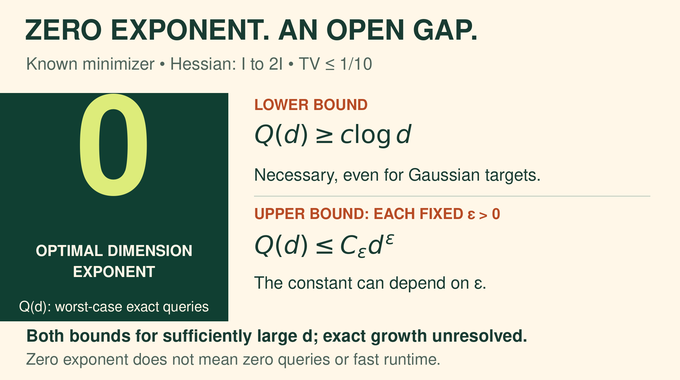
Theorem 1.1 of the sampling manuscript gives, for every fixed , the following bounds once dimension is sufficiently large:
The upper bound also holds for every integer dimension at least two after adjusting the constant. The algorithm may change with the chosen exponent. Smaller exponents can demand larger constants and deeper approximations.
Consequently, the optimal polynomial dimension exponent is zero. This does not identify the exact growth of , or establish a polylogarithmic algorithm. A zero exponent and a matching asymptotic rate are different conclusions.
OpenAI included the work in its public mathematics release. Its Lean formalization scope note states the same normalized assumptions, accuracy, and exponent conclusion, while explicitly excluding arithmetic and bit-cost bounds. That scope is narrower than practical implementation validation, a distinction explored in our guide to mathematical proof formalization.
5. Gaussian Conditioning: Turning Sampling Into a Near-Quadratic Problem
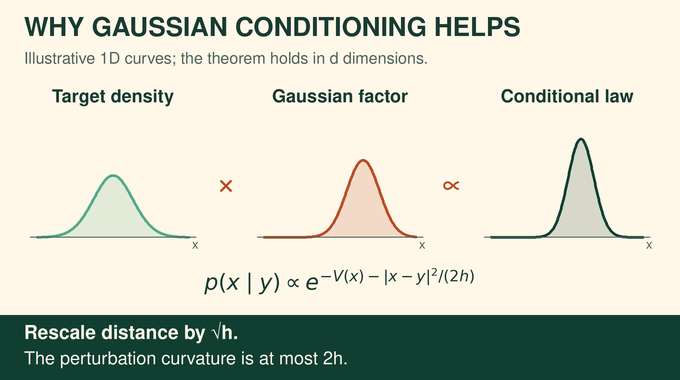
Suppose has the target law and is an independent standard Gaussian. Observe , where controls noise variance. Conditioning on produces:
The observation adds a quadratic bowl centered at . Substitute . The conditional potential becomes , where . Its perturbation gradient has Lipschitz constant at most .
Thus small noise variance makes the rescaled problem nearly quadratic. Each perturbation-gradient evaluation needs just one original-gradient query. The rescaling changes the difficulty of the conditional law without requiring a new information source.
The reusable auxiliary law allows an arbitrary center and a positive scale:
Later centers are random and need not minimize . Uniform control at those centers is essential. A method that only works near the original minimizer would fail when nested inside the rest of the proof.
6. Gaussian Transport and Conditional Gradient Means
For and an independent standard Gaussian , interpolate using . At zero the marginal is Gaussian. As approaches one, it approaches the auxiliary target.
Write and . The marginal laws follow the deterministic transport equation:
This is a flow of probability distributions, not a claim that the original random interpolation paths solve that equation. Their conditional mean velocity supplies the transporting field.
Completing a square shows that evaluating is another auxiliary mean problem, at center and scale . This reuse is elegant but dangerous: a transport algorithm cannot call an unavailable exact expectation for free. Implementing those expectations becomes the central computational obligation.
7. How High-Order Derivatives Become Possible With Only C² Smoothness
The original potential has only two continuous derivatives. Ordinary high-order Taylor reasoning would demand derivatives that may not exist. Gaussian conditioning supplies smooth conditional means instead, so the higher derivatives belong to derived objects rather than the original oracle function.
Smoothness alone is insufficient. A derivative tensor collects many coordinate interactions, and bounding its entries separately can repeatedly introduce powers of dimension. The paper uses a Poincaré inequality to control fluctuations and then bounds cumulant tensors, which encode higher-order dependence.
Its decisive requirement is an all-split bound. Divide a tensor’s coordinate slots into any two nonempty groups and view the result as a matrix. The operator-norm bound must work for every such division. That permits later contractions to be estimated through matrix composition.
Repeated integration by parts then incurs polylogarithmic dimension losses, with one final square-root-of-dimension cost for vector output. This prevents each extra approximation order from adding another dimension power. Stronger accuracy becomes available without assuming that secretly possesses bounded derivatives of every order.
Think of smoothing as moving the differentiation burden from a rough potential onto a Gaussian kernel. The challenge is then quantitative: the resulting derivatives must remain affordable as dimension grows. The all-split estimates supply precisely that control, rather than merely guaranteeing that derivatives exist. Their constants may depend on the fixed derivative order, which the final exponent choice determines.
8. Stationary Centering, Picard Iteration, and High-Order Approximation
Transport handles distributions. Computing a conditional mean with prescribed Gaussian noise requires another construction. The paper couples a smoothed position law to standard Gaussian momentum and builds a flow preserving their product distribution.
A skew-matrix drift makes the position and momentum contributions cancel in the stationary-density calculation. The authors also establish existence of the flow for the required interval. Integrating the momentum equation converts a path integral of gradient means into a Gaussian centered at the desired mean.
This identity initially assumes ideal conditional means and an ideal starting distribution. It is an analytical comparison construction, not yet an executable oracle routine. Keeping that distinction visible prevents the proof from quietly assuming its conclusion.
Picard iteration repeatedly substitutes an approximate trajectory into an integral equation. Polynomial quadrature approximates the resulting integrals. The derivative estimates control these high-order formulas. The proof fixes target error and approximation depth before choosing its mesh, so the formula’s dependency structure does not grow uncontrollably with later numerical choices.
9. The Recursive Noisy-Mean Construction That Makes the Proof Work
Nested means create uncertain centers: an approximate answer from one call becomes the location of the next. Ordinary unbiased estimates do not automatically preserve the correct law through that dependency. The construction instead gives the errors a prescribed Gaussian form.
A seeded routine satisfies a pathwise translation identity. Shifting its center can be compensated by specific shifts of its random seeds, leaving all physical oracle query points unchanged. This is a deterministic identity for fixed seeds, not merely equality of averages.
The proof then reduces the seed covariance before absorbing independent Gaussian center noise. After translating back, the combined seed array has exactly the intended covariance. Without that reduction, the absorbed noise would inflate the variance and implement the wrong law.
There are two depths to control: dependencies inside a finite mean expression and the height of routines evaluating those means. Error and perturbation-size update rules make the recursion terminate. Prescribed query caps hold even for unusual oracle responses or random seeds. This is where formal transport formulas become a finite log concave sampling algorithm.
The final accounting combines a small power cost for each auxiliary call with the number of proximal steps. Both are tuned before execution. Logarithmic overheads can then be absorbed into the requested positive exponent. Finitely many smaller dimensions are handled separately by capped Gaussian rejection sampling, so the asymptotic construction does not leave a hole in the all-dimensions statement.
10. Removing Gaussian Noise to Recover the Original Target Distribution
The auxiliary sampler deliberately outputs a law with extra Gaussian noise. Returning it immediately would miss the theorem’s target. A proximal chain first alternates restricted conditional sampling and Gaussian perturbation, contracting toward the noised target.
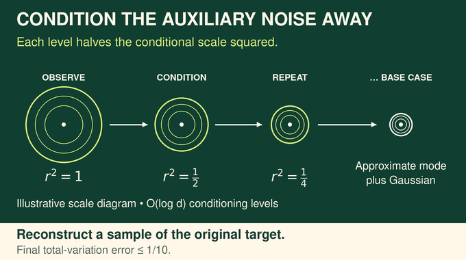
The construction then conditions repeatedly to remove that auxiliary convolution. If an auxiliary sample is observed through , completing the square gives the exact conditional representation:
Each level halves the remaining variance parameter. After logarithmically many levels, the residual conditional law is close to a Gaussian centered at its mode. A capped gradient iteration approximates that mode, and a fresh Gaussian finishes the conditional sample.
Error bounds track random centers using ideal conditioning histories and sum the distributional replacements. The final guarantee concerns the original target, without an additional Gaussian convolution. Carefully recovering the desired marginal also matters in sampling-based approximate counting, although the state space and machinery there are different.
11. Why a Logarithmic Lower Bound Remains Unavoidable
The lower bound already appears for quadratic potentials , with . Their targets are Gaussians with covariance . A gradient reply is , and the value follows from that reply, so each query is effectively one matrix-vector product.
Randomly rotating a carefully chosen spectrum conceals directions from adaptive algorithms. Rotational invariance represents even unrestricted randomized outputs in an enlarged block-Krylov span, formed from Gaussian seed vectors and successive matrix powers. A cosine-based quadratic statistic stays small across that span but has a detectable bias under the target Gaussian. Too few queries therefore cannot reproduce the target distribution.
The lower argument also explains why an easy looking Gaussian is a legitimate mathematical hard instance. Knowing its minimizer immediately reveals its center, but not its covariance. A sampler must learn enough about hidden directional variation to distribute its outputs correctly. Unlimited processing of insufficient oracle information cannot supply the missing directional structure.
This yields a logarithmic necessity, not a matching upper rate. The same need to separate information access from total computation appears in our query-complexity explainer. Here unrestricted real arithmetic can hide substantial work between oracle calls.
For researchers, the constructive opportunity is to understand which smoothing, tensor-control, and noisy-recursion ideas survive realistic computation budgets. For developers, the manuscript supplies no competitive runtime, memory, or stability benchmark. Log concave sampling now has a zero optimal dimension exponent in this precise model, while the gap above logarithmic growth remains open. Follow Binary Verse AI’s research library for explanations that connect theorem statements to their assumptions, mechanisms, and practical limits.
What is log-concave sampling in simple terms?
It is the task of generating random points from a distribution whose log-density is concave. The paper studies how many evaluations of a convex potential and its gradient are needed to obtain an approximately correct sample.
What does subpolynomial query complexity mean?
For every fixed positive exponent epsilon, the theorem guarantees at most a constant depending on epsilon times the dimension raised to epsilon exact value-and-gradient queries. This establishes a zero dimension exponent, but does not prove a polylogarithmic query bound.
What was the previous barrier in log-concave sampling?
Earlier general-purpose methods retained positive powers of dimension in their query bounds under strong convexity and smoothness. The new construction avoids every fixed positive dimension exponent in the specified exact oracle model with unrestricted computation between queries.
Why does OpenAI’s proof use Gaussian conditioning?
Gaussian conditioning produces near-quadratic conditional distributions and smooth conditional gradient means. Those properties support high-order approximation even though the original potential has only two continuous derivatives.
Why does the proof add Gaussian noise and then remove it?
The intermediate noise enables recursive conditional-mean evaluation and error control. A subsequent conditioning procedure removes the auxiliary convolution so the final guarantee applies to the original target distribution.
Does OpenAI’s proof establish the fastest practical sampling algorithm?
No. It bounds exact oracle queries while allowing unrestricted computation between queries. It does not establish superior wall-clock performance, memory efficiency, or numerical stability.
Does the logarithmic lower bound make the query complexity optimal?
Only at the level of the dimension exponent. The optimal exponent is zero, but the precise growth of the minimum worst-case query budget between its logarithmic lower bound and subpolynomial upper bounds remains unresolved.