
A positive solution can look harmless near the origin yet become impossible when the same equations are viewed at larger scales. That contradiction drives OpenAI’s Lane Emden conjecture proof. Its manuscript, dated September 24, 2026, proves that the weighted Hénon–Lane–Emden system has no strictly positive entire solution in the subcritical region, without symmetry, boundedness, or assumptions at infinity. The argument controls localized weighted energy, then shows that dilation would force that energy beyond its universal bound. Here is the theorem’s precise scope, why the weights require extra work, and where the accompanying Lean record stops.
Table of Contents
1. What Did OpenAI Prove About the Lane Emden Conjecture?
The research manuscript’s Theorem 1.1 covers every integer dimension , positive powers , and real weights , provided the weighted subcritical inequality holds. “Entire” means defined throughout Euclidean space. Both functions must be strictly positive, including at the origin.
OpenAI included this work in its October release of mathematical results, described in its mathematics announcement. The manuscript’s September date and the public release date are different events.
1.1. Lane Emden Conjecture Key Facts
| Feature | Precise Scope |
|---|---|
| Dimension | Every integer . |
| Parameters | ; real ; strict subcritical inequality. |
| Regularity | Continuous everywhere; away from the origin. |
| Excluded assumptions | No symmetry, boundedness, stability, global finite energy, or prescribed growth or decay. |
| Conclusion | No strictly positive entire solution in this class. |
This is a Liouville theorem: specified global solutions cannot exist. Setting both weights to zero yields the classical unweighted assertion. The result concerns an exact mathematical system, rather than a numerical search that failed to find a solution.
The distinction between local and global is central. Positive functions can satisfy an equation on a small domain without extending to all of space. The theorem rules out the entire extension under its hypotheses. It does not deny positive solutions on bounded domains with suitable boundary data, and it does not classify sign-changing solutions.
2. The Hénon–Lane–Emden System: Equations and Mathematical Meaning
Here is a point in , and is its distance from the origin. The unknown functions are coupled: each equation’s source depends on the other function. The Laplacian adds second spatial derivatives, measuring local curvature across coordinate directions.
The positive exponents determine nonlinear amplification. The factors introduce position-dependent strength. Positive weights grow outward, while negative weights are singular at zero. Removing them, by taking , gives the Lane–Emden system.
The equations are imposed only away from zero. Continuity there prevents the functions themselves from becoming singular, but does not demand two derivatives at that point. This distinction makes the weighted theorem stronger than a statement restricted to globally smooth solutions. “Positive” also excludes solutions that vanish at the origin, a different admissible class.
3. The Critical Sobolev Hyperbola: Where Solutions Can Exist
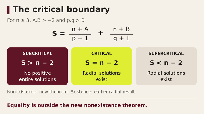
The critical Sobolev hyperbola is the balance line between two scaling regimes. Replacing equality by a strict greater-than sign defines subcriticality here. The terminology describes the exponent region, so relying on “above” or “below” a plotted curve can be confusing.
Its scaling origin becomes visible by assigning dilation powers to the two unknowns. Invariance requires and . Balancing the resulting weighted energy against spatial volume produces the displayed boundary. Section 10 makes that balance explicit.
For the paper’s example , , , the weighted sum is , greater than . Nonexistence follows. Removing the weights at the same powers gives , less than . Weighted subcriticality therefore does not imply unweighted subcriticality.
As a familiar check, equal powers with zero weights reduce the strict condition to for . Equality remains outside the new nonexistence theorem.
4. Why Previous Proofs Could Not Settle the Full Conjecture
Earlier results covered substantial territory. The manuscript traces the unweighted three-dimensional case through growth-restricted results and their removal, then Souplet’s four-dimensional theorem. Higher-dimensional work supplied additional exponent regions. Weighted results included bounded, stable, low-dimensional, radial, and conditional classes.
Those distinctions cannot be erased by calling them all partial solutions. A radial theorem permits reduction to one spatial variable. A boundedness or decay assumption supplies control that an unrestricted positive solution need not satisfy. Neither automatically settles the general higher-dimensional weighted problem.
Two obstacles dominate this paper. Spatial weights anchor the equations to the origin, so translating a solution changes the problem. Moreover, endpoints of weighted source layers do not have constant function values. The new argument retains the weight coefficients in a localized identity and estimates those endpoint variations.
The broader analytical theme is obtaining estimates from the equation itself. Readers of our local smoothing conjecture explainer will recognize the importance of precise regularity and exponent ranges, although the equations and proof mechanisms differ.
There is also a logical danger in assuming finite total energy in order to justify a global identity. Such an assumption could exclude exactly the hypothetical solutions the conjecture asks about. Localization avoids this circularity: every integral used initially is finite for each candidate on a compact region, while uniform control is proved later.
5. First Reductions: Dimensions, Singular Weights, and the Condition pq > 1
The proof assumes a positive solution and progressively removes impossible cases. Lemma 2.1 averages each function over spheres centered at zero. The equations make the corresponding radial flux strictly decreasing. Continuity at zero forces its limiting value there to vanish.
In dimension two, integrating the negative flux eventually forces a spherical mean below zero. If , positivity of near zero forces curvature strong enough to violate continuity of . Interchanging the equations excludes . Thus any candidate requires and . These are deductions, not extra assumptions added to Theorem 1.1.
Lemma 2.2 extends the equations across zero in the distributional sense and establishes potential representations up to nonnegative constants. Lemma 2.3 then compares the infima of on centered balls. If , the equations force an increasing power of the radius to remain below a fixed bound. Letting the radius grow is impossible. Only remains.
Spherical averaging does not impose radial symmetry on the original functions. It extracts consequences shared by every solution, even one with strong angular variation. The later proof returns to the full spatial functions. This is why an argument using spheres can still establish a theorem for unrestricted, nonradial solutions.
6. Newton Potentials and Origin-Centered Scaling
Write and . The Newton kernel is , where and the sphere factor denotes surface area. Convolution with this kernel reconstructs a function from its source.
Proposition 2.4 removes the possible additive constants and gives the exact identities , away from zero. For , define
Then and satisfy the same equations. Both exponents are positive after the reductions.
The proposition bounds centered source masses by and , with centered at zero. Here depends on equation parameters, not the solution. These estimates control distant potential contributions. A small ball elsewhere is handled by containment in a fixed centered ball, never by translating the weighted equation.
A universal bound differs from a solution-dependent one. Continuity already makes each candidate bounded on a compact ball, but its maximum could depend on the candidate. Scaling would then offer no contradiction. Proposition 2.4 instead fixes constants using only the equation’s parameters, creating estimates that survive unchanged when the candidate is dilated.
7. The Localized Virial Identity: Preserving the Spatial Weights
The potential formulation defines a nonnegative interaction measure
Integrating out gives ; integrating out gives . A compact cutoff equals one on the unit ball and vanishes outside radius two. Set , a nonnegative annular weight, and .
The localized energies are , , and . With , , integration by parts produces coefficients and . Keeping those weight-dependent terms is essential.
Lemma 3.2 compares the two energies and approximates the interaction by its radial-direction contribution. Its total error is at most , for any positive . This does not assume that is uniformly bounded. It makes the error absorbable once a positive subcritical coefficient appears. The cutoff’s high-order vanishing prevents its boundary derivatives from overwhelming that estimate.
The interaction uses , a kernel-adapted difference quotient. The exact identity is
Compact support removes a boundary contribution at infinity. The origin contribution vanishes using the already established weight restrictions. These are the specific justifications that allow integration by parts despite the theorem’s weak assumptions.
8. The Interval-Pair Inequality: A Geometric Step in the Proof
Lemma 4.1 temporarily leaves the equations behind. Take two distinct parallel lines and an interval on each. Restrict the Newton kernel to pairs of points on those intervals. The kernel depends on their transverse separation and longitudinal difference.
Integration by parts compares the average interaction with kernel values at interval endpoints. A directional correction measures how much of the separation lies along the lines. Unequal nonnegative interval weights contribute an additional mismatch term.
Why does the midpoint calculation work? The distribution of longitudinal differences is symmetric around the difference of the two midpoints. Its density is an interval-overlap length, decreasing with distance from that center. Pairing positive and negative differences gives the sign needed for the correction estimate.
This converts bulk interaction into endpoint information, precisely what source layers will provide. The lemma is also stated using nonnegative integrals. An unbounded interval with zero weight needs no endpoint evaluation. That care matters in dimension three, where individual line integrals can diverge and subtracting two infinities would invalidate the argument.
9. Weighted Source Layers and Angular Localization
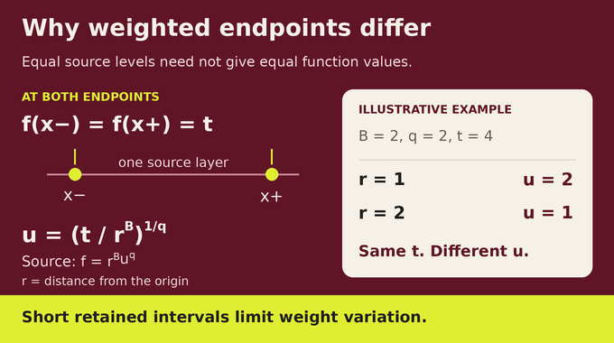
A source layer is a superlevel set such as . Intersecting it with a line produces intervals. At a finite endpoint , the source equals , but the function equals . Unlike the unweighted case, equal source levels do not give equal endpoint values.
Section 5 resolves this by averaging directions inside small caps around the local radial direction. Each retained interval receives a constant weight, chosen as an infimum along that interval. Only bounded, sufficiently short intervals retain positive weight. Their endpoint spatial factors consequently vary little.
Discarding intervals costs something. A polar-integration argument bounds the probability that a source layer contains a long segment. Splitting levels into high and low parts converts that probability estimate into a small energy-relative loss plus a universal constant.
The proof chooses cap width first, interval tolerance second, and the layer threshold last. Combining their errors yields Proposition 5.1, the localized pressure inequality. Its pressure term is a directional kernel integral, not a physical fluid pressure. Crucially, its error remains before any universal energy bound is known.
Writing , the pressure estimate reads . Here is the squared cosine between the separation vector and the radial direction at . Averaging the cap weights recovers the original annular weight exactly, while their directional error is absorbable. Thus the geometric lemma returns precisely the term needed by the virial identity.
10. The Final Proof: Uniform Energy Bounds Versus Scalingy
Let . The theorem assumes . The virial identity and pressure inequality combine, while the marginal estimate replaces the difference between and by another controllable error.
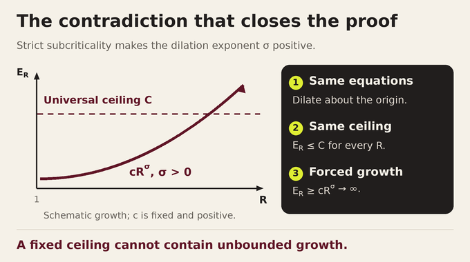
Choosing small relative to absorbs every energy-relative term into the left side. Proposition 6.1 follows: the weighted energy on the unit ball has a universal upper bound. The constant may depend on the parameters, but is identical for every admissible solution and every dilation.
Here are the sources of the scaled functions. Positivity makes the integral over the unit ball strictly positive. For , the larger-ball integral is at least that fixed amount. Multiplication by therefore forces divergence, contradicting the uniform bound. The identity , with , explains exactly why strict subcriticality supplies the contradiction.
No assumption about finite energy over the whole space enters this last step. Each finite-radius integral exists, and a fixed inner ball supplies a positive lower bound. That is enough: a growing dilation factor already contradicts a constant upper bound. The proof never needs to calculate the hypothetical solution’s total energy.
11. What Happens on the Critical Hyperbola? Phan’s Conjecture C
At equality, the scaling exponent used above is zero. The contradiction disappears. Corollary 6.2 instead combines the new nonexistence theorem with the earlier radial ground-state theorem of Bidaut-Véron and Giacomini. For , , and positive powers, that theorem provides positive entire radial solutions when the subcritical inequality fails.
11.1. Existence and Nonexistence Classification
| Weighted Sum S | Region | Positive Entire Solutions |
|---|---|---|
| Subcritical | None in the stated class, by the new theorem. | |
| Critical | Radial solutions exist, by the earlier existence theorem. | |
| Supercritical | Radial solutions exist, by the earlier existence theorem. |
Here . Existence of a radial solution establishes existence in the unrestricted class too. It does not assert that every solution is radial. The combined classification settles Phan’s Conjecture C in this admissible range; it does not extend the existence assertion to arbitrary real weights.
The equality case therefore has a different evidential route from strict subcriticality. Calling the whole classification a newly constructed family of solutions would misattribute the older work. The new contribution eliminates the remaining positive solutions in the forbidden region, allowing the established existence theorem to complete the picture.
12. Lean Verification, Mathematical Significance, and Remaining Limits
OpenAI’s published Lean scope note identifies the strict subcritical nonexistence theorem as formalized, including the unweighted case. It explicitly excludes critical equality. The existence classification therefore should not be described as entirely covered by that note.
Formal checking validates a precise encoded statement. Assessing its correspondence with the manuscript, the exposition, and novelty requires additional mathematical judgment. The public sources checked here do not establish a journal peer-review verdict, and this article does not rerun Lean. Our Fermat formalization explainer and Navier–Stokes proof-scope guide explain why those distinctions matter.
For researchers and students, the practical value is a reusable chain of estimates and a precise theorem to consult in related elliptic problems. The manuscript situates Liouville theorems within rescaling arguments for bounds and singularity estimates. It does not demonstrate a faster numerical solver or a new engineering application.
The Lane Emden conjecture result supplies a global nonexistence theorem under unusually weak assumptions. Its transferable idea is controlling weighted localization errors relative to an energy before bounding that energy. Potential uses in other systems remain a research direction. For more source-led mathematical explanations, explore Binary Verse AI’s ionization conjecture analysis and follow our growing research reference series.
Has the Lane–Emden conjecture been solved?
OpenAI’s September 24, 2026 manuscript proves subcritical nonexistence for the classical Lane–Emden system and its weighted Hénon extension in the stated positive entire solution class. For and , combining that theorem with an earlier radial existence result gives the corresponding existence and nonexistence classification. The manuscript’s claim, its declared formalization scope, and independent peer review remain distinct forms of evidence.
What is the difference between the Lane–Emden and Hénon–Lane–Emden conjectures?
The classical Lane–Emden system has no spatial weights: and . The Hénon–Lane–Emden system includes and in the respective source terms. These factors change the critical condition, anchor the equations to the origin, and require weighted estimates.
What is the critical Sobolev hyperbola in the Lane–Emden system?
It is the boundary . Replacing equality by a strict greater-than inequality defines the subcritical region of the nonexistence theorem. In the unweighted case, set .
Does the OpenAI proof require radial symmetry or bounded solutions?
No. Theorem 1.1 assumes neither radial symmetry nor boundedness, stability, integrability, global finite energy, or prescribed growth or decay at infinity. It requires both functions to be continuous and strictly positive everywhere, and away from the origin, where they satisfy the equations.
Why does the weighted Hénon–Lane–Emden case require a new argument?
Spatial weights break translation invariance and make function values at source-layer endpoints depend on their position. The manuscript uses origin-centered source estimates, caps around radial directions, short retained intervals, and controlled discarded-layer losses to obtain a localized weighted pressure inequality.
What happens at the critical and supercritical boundaries?
The new theorem establishes nonexistence only in the strictly subcritical region. For , , and , the earlier radial existence theorem supplies positive entire solutions at critical equality and in the supercritical region. This does not mean that every solution there must be radial.
Has OpenAI’s Lane–Emden proof been formally verified in Lean?
OpenAI reports a Lean formalization of the principal strict subcritical nonexistence result, including the unweighted case. Its scope note explicitly excludes critical equality. This article has not rerun the formal proof. Formal checking of an encoded theorem and independent expert review of the manuscript are different forms of validation.