
Seven dots, twenty-one connections, nine unavoidable crossings. That is the answer for the complete graph , even when every connection may bend. The difficult question was whether the same classical formula remained optimal for every graph size, however cleverly its edges were routed.
OpenAI’s September 23, 2026 paper presents a proof that the crossing number of complete graphs equals the Harary–Hill floor-product formula. Its argument supplies the missing universal lower bound, then matches it with a two-page drawing. OpenAI also reports a Lean formalization with both components in its stated scope. Here is how the proof turns intersections into polynomial information, and that information into an exact minimum.
Table of Contents
1. What Is the Crossing Number of a Complete Graph?
A complete graph connects every pair of its vertices, giving edges. Vertices are distinct points. Edges are simple continuous arcs whose interiors avoid vertices. Different edge interiors meet only at finitely many proper double crossings, with no overlaps, tangencies, or triple intersections.
For a drawing , let count its crossing points. The ordinary crossing number is the smallest such count over all admissible plane drawings. If two edges cross three times, that contributes three, rather than one. Shared endpoints are vertices, not crossings.
1.1. Crossing Number of Complete Graphs: Key Facts
| Question | Answer |
|---|---|
| Graph family | has vertices and one edge for every vertex pair. |
| What is minimized? | The total number of interior crossing points across all ordinary plane drawings. |
| Are curved edges allowed? | Yes. Edges are simple continuous arcs. Repeated crossings between two edges count separately. |
| What does the paper prove? | The Harary–Hill floor product is the exact minimum, with a matching two-page construction. |
| What is the formal scope? | OpenAI reports both the lower bound and the matching construction in Lean. |
The crossing number of a complete graph concerns the best drawing, rather than the first picture generated by a layout tool. is the first complete graph that cannot be drawn without a crossing. Its ten edges exceed the nine-edge maximum for a planar graph on five vertices, while a one-crossing drawing exists.
2. The Harary–Hill Formula: Exact Crossings for Every Kₙ
Theorem 1.1 of the complete-graph crossing paper states, for every integer :
The floor function means the greatest integer no larger than . Thus . The complete graph crossing number formula multiplies four such integers and divides by four. The result is an exact minimum because the paper proves both that every drawing needs at least this many crossings and that a drawing attains it.
Our bin packing explainer similarly separates a feasible construction from proof of the true optimum.
2.1. Minimum Crossings for Small Complete Graphs
| Complete Graph | Minimum Crossings |
|---|---|
| 1 | |
| 3 | |
| 9 | |
| 18 | |
| 36 |
For the crossing number of , the calculation is . For the crossing number of , it is . Adding a vertex can increase the minimum sharply because it introduces an edge to every existing vertex.
3. Why the Harary–Hill Conjecture Resisted Proof for Decades
Hill’s construction was known long before this manuscript. Guy published an upper bound in 1960, and Harary and Hill discussed the construction and conjecture in 1963. But an attractive drawing answers an existence question: can this count be achieved? Optimality asks whether every conceivable drawing must do at least as badly.
Earlier work established exact small cases. The paper cites computer-assisted results giving 100 crossings for , 150 for , 225 for , and 315 for . The earlier two-page crossing theorem also established the formula within that restricted drawing class. Shellability extended the lower bound to additional families, without covering arbitrary drawings.
Balogh, Lidický, and Salazar’s asymptotic lower-bound research pushed the limiting ratio to the conjectured value above 0.98559895, or 98.559895 percent. An asymptotic percentage cannot establish exact equality at every size. As with Boolean-circuit lower bounds, every permitted representation must be covered. A Harary–Hill conjecture proof needed unrestricted reach. OpenAI extracts algebraic constraints that every drawing must obey.
4. Hill’s Two-Page Drawing: A Construction That Achieves the Formula
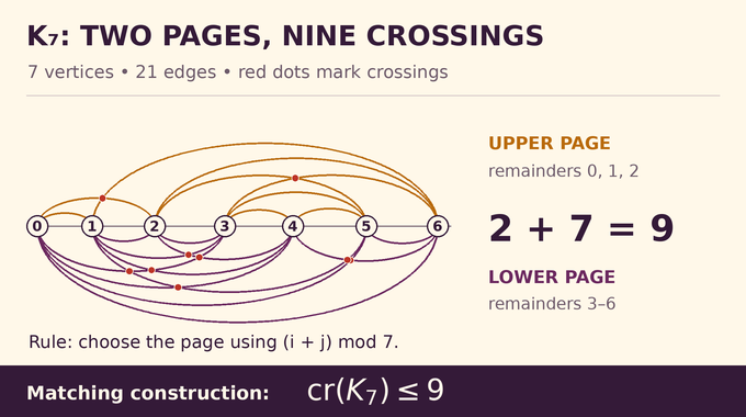
Section 5 uses an endpoint-sum book construction attaining Hill’s classical bound. Number the vertices from 0 to and place them left to right on a horizontal spine. Set . Assign residues 0 through to the upper page and the remaining residues to the lower page.
For an edge joining and , reduce modulo and choose the corresponding page. Draw it as a semicircle there. Edges on opposite pages cannot cross. On the same page, two edges cross exactly once when their four endpoints alternate along the spine. Nested endpoint intervals do not produce crossings.
For , residues 0, 1, and 2 go above the spine. This gives two crossings above and seven below. For example, edges 02 and 16 belong above and cross because . Choose vertex positions generically to prevent triple intersections. The paper’s enumeration, including a parity check for even orders, gives exactly . This proves .
5. Why the Proof Can Start With Normalized Drawings
Curved edges need careful handling before tangent signs and local orders become useful. Appendix A proves that a minimum drawing can be chosen polygonal, straight near vertices and crossings, and free of crossings between adjacent edges. Adjacent edges share a vertex.
The argument isolates vertices and crossing points inside disjoint small disks. Between disks, retained edge pieces sit inside separate neighborhoods. Each continuous piece can be replaced by a polygonal path within its neighborhood, so replacements cannot accidentally collide. Inside crossing disks, straight chords introduce at most one crossing. Inside vertex disks, straight spokes meet only at the vertex.
Crucially, the construction cuts away passages using first and last visits to the disks. It does not assume a continuous arc visits a circular boundary only finitely often. This closes a subtle gap that an informal “straighten everything” instruction would leave.
If adjacent edges crossed in a minimum drawing, swapping their initial tracks and removing loops would eliminate a crossing without adding another. That contradicts minimality. Independent edges may still cross repeatedly. Normalization therefore prepares the geometry without silently changing the objective to counting intersecting pairs.
6. Signed Intersections and the Cycle-Pairing Identity
Orient each edge. A crossing receives sign +1 or −1 according to whether the ordered tangent directions agree with the plane’s positive orientation. Write for the sum of these signs. Unlike the ordinary crossing count, this sum permits cancellation.
At a vertex , list incident edges counterclockwise from a chosen gap. Let be +1 when precedes , −1 for the reverse order, and zero when they coincide. Let be +1 for an edge pointing outward and −1 for one pointing inward. The corrected pairing is:
A cycle is an edge combination with zero boundary: incoming and outgoing coefficients balance at each vertex. Lemma 2.1 proves that for any two cycles. Geometrically, closed walks have total signed intersection zero in the plane. When cycles share vertices or tracks, averaging two slight displacements produces the half-weight correction. The local term makes the geometric cancellation valid even with shared edges. This pairing is skew-symmetric: exchanging its arguments reverses its sign.
7. Lagrange Interpolation and the Even-Node Order Detector
Give vertices distinct real labels, separate from their positions in the drawing. For distinct nodes , define . Lagrange interpolation supplies the weighted identity:
It follows by comparing the highest-degree coefficient in the interpolation formula. The denominators are nonzero because the nodes are distinct. These weights later make suitable polynomially weighted edge combinations into cycles.
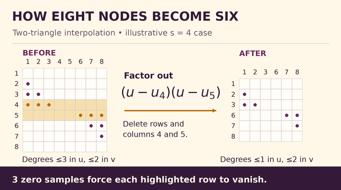
For nodes, Lemma 3.2 samples a two-variable polynomial on two triangular patterns of index pairs. In the first half, select ; in the second, select . Together the patterns contain points. They determine polynomials of separate degrees at most , or the swapped limits.
For eight nodes, rows 4 and 5 each contain three samples. A polynomial of degree at most two in its second variable must vanish along both rows if those samples vanish. Dividing out leaves the smaller six-node problem with the degree limits swapped.
Lemma 3.3 combines this interpolation with the prescribed local order. Its pairing includes order signs, node differences, and Lagrange weights. Weighted cancellation removes allowable row and column terms, leaving nonzero diagonal weights on the two triangles. Thus the detector is nonsingular for any prescribed order, even when that order differs from the numerical order of the labels.
“Nonsingular” means that a polynomial cannot hide from every test polynomial unless it is zero. The geometry chooses the local order, while the labels can be arbitrary distinct real numbers. Requiring those two orders to agree would impose an unjustified restriction on the drawings. The detector avoids that restriction, which is why this interpolation lemma can serve a universal lower bound.
8. Why the Crossing Evaluations Determine the Polynomial
Now take , with . Let contain four-variable polynomials of degree at most in each variable. Require symmetry within and within , but not under exchanging the two edge pairs.
A symmetric polynomial in one pair has a basis indexed by exponent pairs . There are choices. Choosing a basis element independently for each endpoint pair gives:
Let be the ordered pairs of independent undirected edges with nonzero signed crossing count. Evaluate each polynomial at the four vertex labels of every pair in . This defines . Injectivity means that zero evaluations force the entire polynomial to be zero.
Lemma 4.2 assumes all those evaluations vanish. Polynomial cycle tests eliminate independent-edge terms. Additional factors eliminate all but one shared-endpoint pattern, while interpolation isolates individual vertices. The order detector then forces vanishing whenever endpoints from different edges coincide.
Consequently, all four cross-edge difference factors divide the polynomial:
Their product is nonzero on independent-edge evaluations. The quotient retains both symmetries, remains in , and still has zero evaluations, but its separate degrees are two smaller. Choosing a nonzero kernel polynomial of minimum degree makes this impossible. Therefore is injective: crossing evaluations retain all the polynomial information the argument needs.
9. The Dimension Argument That Forces Unavoidable Crossings
Injectivity alone does not count crossings. Proposition 4.3 applies the cycle tests again, now multiplying two polynomials by all six endpoint differences:
For , each variable in has degree at most , exactly within the cycle-test limit. A shared endpoint makes zero. Only supported independent-edge coordinates remain.
The resulting identity defines a nondegenerate symmetric diagonal bilinear form on . This is different from the earlier skew-symmetric pairing . Each diagonal coefficient is nonzero. Reversing the order of the two edges gives a separate coordinate with the opposite coefficient, allowing cancellation without degeneracy.
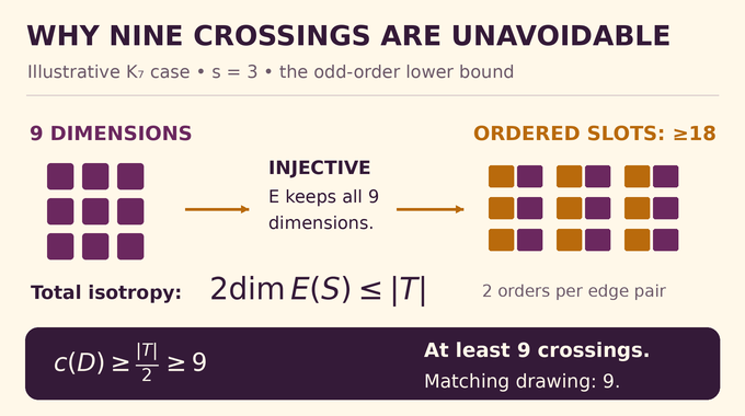
The image is totally isotropic: every pair of its vectors has pairing zero, including a vector paired with itself. Hence . Nondegeneracy gives , so:
Each supported unordered edge pair needs at least one actual crossing. Ordered pairs count it twice. Combining this observation with injectivity gives:
Repeated crossings can cancel in the signed sum and remove coordinates from . That only reduces the support being counted. It cannot invalidate the lower bound on actual crossing points.
For , take . The polynomial space has dimension nine. Injectivity preserves those nine independent directions, while total isotropy requires at least eighteen ordered support coordinates. These represent at least nine unordered crossing pairs. The construction from Section 4 reaches nine, so the algebraic count and the visible drawing agree.
10. Extending the Proof From Odd to Even Complete Graphs
Odd order leaves an even number of other vertices around each vertex, matching the detector’s nodes. For even , the paper transfers the odd bound by deleting each vertex in turn.
Every crossing in a normalized minimum drawing involves four distinct vertices. It survives deletion of precisely the other vertices. Each remaining drawing of has at least the odd-order minimum, regardless of whether that particular subdrawing is optimal. Summing gives:
Rearranging produces , the even-order floor product. For odd order, the value is . The cases need only the nonnegative lower bound and crossing-free constructions. Both parity arguments therefore support the same compact formula, rather than two unrelated answers.
11. What OpenAI’s Proof Establishes and Why the Bounds Match
The lower bound applies to unrestricted ordinary drawings. The two-page construction supplies the matching upper bound:
OpenAI’s mathematics release announcement attributes the wider collection of AI mathematical proofs to an internal frontier model. That context does not supply a paper-specific runtime or reproducible public-model workflow. LLM math benchmark scores measure different evidence. Unlike an algorithmic result such as maximum cardinality matching, this determines an optimum without demonstrating faster graph-layout software.
As checked on October 30, 2026, OpenAI’s Lean scope documentation includes the exact formula, lower bound, and matching two-page drawing. The linked complete-graph comparator specifies a target theorem with a placeholder, rather than providing the implementation proof. This article did not independently rebuild the Lean project. Formal statement fidelity and expert review of the exposition remain separate checks.
The OpenAI Harary–Hill proof concerns ordinary crossing numbers. Straight-line drawings form a restricted subclass, so the formula supplies a lower bound there without establishing rectilinear equality. Pair-crossing and odd-crossing objectives also require separate statements. For the crossing number of complete graphs, the achievement is precise: construction and necessity finally meet. Follow Binary Verse AI for research explainers that connect theorem statements to the arguments and verification evidence behind them.
How do you calculate the crossing number of a complete graph?
For a complete graph , substitute into the Harary–Hill formula and evaluate its four floor factors. OpenAI’s paper proves that the result is the exact minimum over all ordinary plane drawings, rather than merely the crossing count of one construction.
What are the crossing numbers of K5, K6, and K7?
They are 1, 3, and 9, respectively. For , the formula gives . These are the minimum crossing counts when edges may be continuous curves.
Why is K5 nonplanar, and how many edges does it have?
has ten edges. A simple planar graph with five vertices has at most edges, so cannot be drawn without crossings. A drawing with exactly one crossing exists, giving .
Why did Hill’s original construction not settle the conjecture?
It supplied drawings attaining , which proved an upper bound. It did not exclude every drawing with fewer crossings. The missing step was a matching lower bound without restrictions on vertex positions or edge routes.
How does polynomial interpolation prove a geometric crossing bound?
The proof converts signed intersection and local-order information into polynomial identities. An interpolation-based detector makes the evaluation map injective. A second identity puts its image inside its orthogonal complement for a nondegenerate symmetric form. Comparing dimensions then forces enough supported edge pairs, and therefore enough crossings.
Does the proof apply to curved edges and straight-line drawings?
It applies to unrestricted ordinary drawings with simple continuous curved edges, counting repeated crossings separately. Straight-line drawings are a restricted subclass, so the theorem supplies a lower bound for their crossing numbers. It does not establish equality for the rectilinear crossing number.
Was OpenAI’s Harary–Hill proof verified in Lean?
OpenAI reports a Lean formalization whose stated scope includes the exact complete-graph crossing formula, the lower bound, and a matching two-page construction. The linked comparator defines a target theorem with a placeholder and is not itself the implementation proof. This article did not independently rebuild the project. Machine checking of an encoded statement and review of the accompanying natural-language exposition are distinct checks.