
Remove less than one percent of a unit interval. Can the remaining compact set exclude every translated, stretched, compressed, or reflected copy of an infinite geometric progression? OpenAI’s proof answers yes for every fixed ratio . Its October 5, 2026 paper establishes the geometric case of the Erdős similarity conjecture: however small the permitted loss of measure, an avoiding set exists. The set may depend on the ratio. This does not settle the conjecture for arbitrary infinite sets, and the available Lean formalization covers the dyadic ratio .
The surprise is structural: preserving nearly all the interval does not preserve every infinite pattern. The original geometric-case paper explains how carefully coordinated random tests make that possible.
Table of Contents
1. What Is the Erdős Similarity Conjecture?
Lebesgue measure gives the usual length of measurable subsets of the real line. A measure-universal set has an affine copy inside every measurable set of positive measure. Here , with . Translation chooses the location, dilation changes size, and a negative dilation also reflects the pattern.
Erdős’s 1974 problem asks whether any infinite set can be measure universal. The conjectured answer is no. To disprove universality for one pattern, it suffices to construct one positive-measure set avoiding every affine copy. “Almost full” means a much stronger quantitative guarantee within , rather than full measure or the presence of an interval.
| Question | Paper’s Answer |
|---|---|
| Pattern | , with one fixed ratio. |
| Avoiding Set | Compact, inside the unit interval, arbitrarily close to full measure. |
| Transformations | Every real translation and every nonzero signed dilation. |
| Proof Method | Finite random routing, local scale counts, open-set repair. |
| Formalization | Dyadic case only in the supplied Lean scope document. |
2. Why Finite Patterns Are Unavoidable but Infinite Ones Are Different
For a finite pattern, choose a bounded measurable target of positive measure. Translating that target by a sufficiently small amount changes it only slightly in measure. For finitely many translated targets, the total loss remains small, leaving a positive-measure intersection. Any point in that intersection supplies a translation placing the suitably shrunken pattern inside the target.
This uses continuity of translations in the space of integrable functions. It also explains why allowing arbitrarily small nonzero dilations matters: an interval is unnecessary, even when the target is fragmented.
For infinitely many points, however, finitely controlled losses can accumulate. An argument handling every finite prefix separately need not produce one translation and one scale that work for the entire sequence. Each longer prefix may require different parameters. The theorem exploits precisely that distinction. Questions of length and geometry also meet in the Kakeya problem, although its patterns and quantifiers are different.
3. The Previous Obstacle: Why Geometric Sequences Resisted Earlier Proofs
The paper credits Falconer and Eigen with nonuniversality results for decreasing positive sequences approaching zero whose successive ratios tend to one. A geometric sequence instead has a constant ratio below one, so those results do not apply.
Another criterion examines arbitrarily large finite subsets: the negative logarithm of their minimum gap divided by their total span must be as their cardinality grows. Distinct geometric powers have normalized minimum gap at most . Its negative logarithm grows at least linearly, defeating that sufficient criterion.
Additive results are also different. Avoiding a sum or difference involving a geometric sequence does not imply avoiding that sequence alone. A larger pattern is easier to obstruct because destroying one required point already destroys its complete copy. Readers exploring other additive-pattern questions can compare the Hindman finite-sums problem. The unresolved task here was to obstruct the single geometric progression itself.
4. OpenAI’s Theorem: An Almost-Full Set That Avoids Every Affine Copy
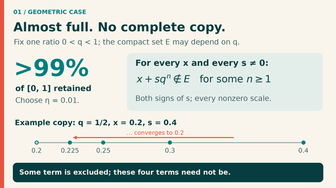
Theorem 1.1 fixes and . It constructs a compact set inside satisfying:
For every real center and every , at least one point lies outside that set. Both signs of dilation are included. The exponent is a positive integer and can depend on the proposed copy.
Take . More than 99 percent of the interval remains, yet no complete affine copy of the chosen geometric sequence survives. “Paradox” describes the tension with intuition, not a contradiction in measure theory. The deleted points are coordinated across positions and scales.
The quantifier order matters: choose a ratio, then build its avoiding set. The theorem supplies such a set for every fixed ratio, but does not supply one set working simultaneously for all ratios. These are different mathematical statements.
For a concrete dyadic copy, take center 0.2 and dilation 0.4. Its first points are 0.4, 0.3, 0.25, and 0.225, converging to 0.2. The theorem guarantees that some point of this infinite list is excluded. It does not identify which of these first four points, if any, must be missing. A finite numerical check cannot establish the required infinite avoidance.
5. The Key Reduction: Turning Avoidance into a Periodic Hitting Problem
Rather than construct the retained set directly, Proposition 2.1 builds a small open set that every normalized copy must hit. It repeats with period one. For any probability parameter , its density obeys:
Density means the measure occupied in one period. The proposition requires, for every center and every , some to belong to . The final avoiding set will be the complement of suitably rescaled hitting sets.
This reverses the design task: every proposed infinite progression needs only one missing point. Periodicity handles all spatial locations using one finite grid model per period. Restricting scales to a compact interval makes boundary counting possible. Later, powers of two and reflections recover arbitrary nonzero dilations without requiring any special algebraic relationship between two and the ratio.
6. Nested Dyadic Grids and Preorder Windows: Preparing Independent Tests
Section 3 sets and defines dyadic grid resolutions by:
Here the ceiling rounds upward, giving . Powers of two make the grids nested. The periodic key records a point’s cell, where braces denote fractional part. Cells include their left boundary and exclude their right boundary.
Each edge of an ordered tree receives an index window . Preorder lists an edge before its entire child subtree. Consecutive windows have unused indices between them. At height , windows have length . Lemma 3.1 bounds the edge-and-subtree span, with its last endpoint:
Lemma 3.2 calls centers stable when relevant rightward translations cross no earlier grid boundary. Large gaps make unstable centers rare. Lemma 3.3 separately proves that translated points within one window, and the center, have distinct current-grid keys. Stability preserves old decisions. Separation provides fresh entries.
These two properties operate at different resolutions. A later window supplies tiny translations, small enough to preserve an earlier coarse key. Its own grid is much finer, so those same translated points are distinguishable there. The initial index is chosen so all displacements lie within a quarter of a period, preventing circular wraparound from defeating the distance estimates.
7. The Random Routing Tree: How the Construction Creates Fresh Tests
The tree has children per internal vertex and depth . Each nondefault edge carries an independent table of fair selector bits. A point follows the first child whose addressed bit is one. If all earlier selectors are zero, it takes the final, default child.
Each leaf has a separate table of independent Bernoulli- bits: one occurs with probability . Membership in the random periodic set is decided by the addressed terminal bit. Lemma 4.1 therefore gives expected density , regardless of the routing complexity.
Expose the center’s entry in every selector table, forming the information field . On a fixed exposure outcome , its route and first default vertex are known. Lemma 4.2 uses stability to preserve the translated points’ earlier choices. A successful test through a nondefault child of therefore certifies actual membership in . This implication prevents counting apparent hits that routing would bypass.
A default is useful because all the center’s earlier child selectors at that vertex are known zeros. Nearby test points can now try those children using fresh entries. Branching supplies more opportunities, while terminal probabilities keep the expected amount removed small. The design separates the number of opportunities from the density charged for membership.
8. The Probability Calculation: Why Missing a Pattern Becomes Unlikely
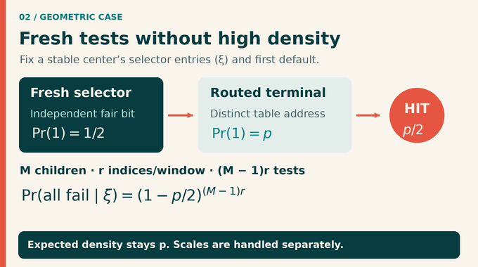
At the first default vertex, the nondefault children supply tests. Lemma 4.3 fixes one scale and conditions on the center exposure. Its exact probability that all tests fail is:
The reasoning has two stages. Separation makes the newly queried selectors independent fair bits, untouched by the exposed center entries. Then conditioning on all selectors fixes every test’s terminal address. Those addresses are distinct, including when tests reach the same leaf, because finer grids preserve their different keys. Thus terminal entries are independent Bernoulli- variables. Averaging over selectors produces the displayed expression.
This establishes conditional independence at a fixed scale. It does not assert independence between scales. Separately, the probability that the center’s route has no default is . Increasing tree depth makes that possibility small, ensuring the construction usually obtains its family of tests.
9. The Decisive Step: Controlling Every Scale Simultaneously
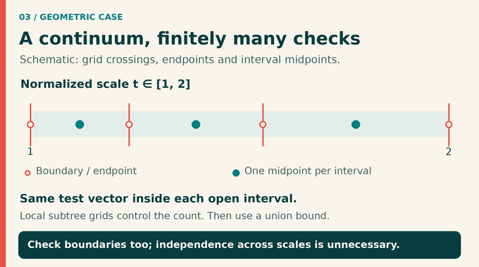
Lemma 5.1 replaces the continuum of normalized scales by finite representatives. For each local test, record scales where a translated point crosses its relevant finest grid boundary. Include those boundary scales, both endpoints, and a midpoint between consecutive boundaries. The entire test vector is constant on each intervening open interval.
The representative count is at most , where:
A union bound, rather than independence across scales, bounds the probability of some missed scale by . Here is the natural logarithm. The paper chooses branching large enough that:
This makes the failure decay beat representative growth as window lengths increase. Crucially, the count uses the last grid of each edge’s child subtree. The span inequality controls that resolution locally. Using the whole tree’s finest grid would lose this advantage. This local accounting is the mechanism that closes the geometric case, not an unrestricted claim that enough random trials handle any continuum.
Boundary representatives are essential. Sampling only interval midpoints would ignore possible changes exactly where a translated point reaches a cell boundary. Keeping each boundary separately respects the half-open convention. The representative list is fixed under the center exposure before the remaining random entries are revealed, so applying the fixed-scale estimate to every listed value is justified.
10. Repairing Exceptional Centers and Building the Almost-Full Compact Set
The parameters are chosen in order: branching, depth, index gaps, then minimum window length. The proof bounds missed-scale probability at stable centers by twice . Enlarge selected cells into an open periodic set, then let contain centers still missed at some normalized scale. Integration over centers bounds its expected density by three times .
Choose an outcome whose enlarged-cell density plus exceptional-center density is at most five times . Cover by an open periodic neighborhood, spending another . This yields the density budget. At exceptional centers, late translated points enter that neighborhood because they converge to the center. These repair indices need not belong to the original finite windows.
This repair changes a statement about each center’s probability of failure into one construction valid at every center. The exceptional set is closed because it is obtained by projecting a closed subset of a compact center-and-scale space. An open neighborhood can therefore cover it with arbitrarily little additional measure. Convergence then supplies the actual hit, including at centers the finite tests missed.
For the global step, use and corresponding hitting sets in:
The paper obtains . Consequently is compact and has the required measure. Positive scales normalize through . Reflections handle negative scales. Summability pays for both expanding and contracting copies.
11. What the Geometric-Case Proof Establishes and What Remains Open
For , the sequence is one half, one quarter, one eighth, and so on. Every proposed translated and nontrivially scaled copy loses some point from the constructed set. This includes arbitrarily small scales and reflected copies. The general-ratio theorem gives the corresponding conclusion separately for every ratio strictly between zero and one.
It does not settle the full Erdős similarity problem. Nor does avoiding a complete infinite progression mean avoiding all its finite prefixes. Every finite pattern remains measure universal. The theorem also concerns affine maps, which preserve relative spacings, rather than arbitrary deformations.
The paper explicitly contrasts affine avoidance with bi-Lipschitz embedding results. Such maps may distort distances within fixed multiplicative bounds, while an affine copy uses one common scale for every pair. Allowing that extra flexibility changes the embedding question. Likewise, full Hausdorff dimension alone cannot substitute for the positive Lebesgue measure required here.
The result is an existence theorem. It supplies no practical runtime benchmark for producing usable avoiding sets. Its finite probability spaces support the proof, but finiteness alone supplies no efficiency guarantee. The same distinction between a mathematical result and measured performance matters when reading LLM mathematics benchmarks.
12. Formal Verification and the Value of a Scoped Result
OpenAI’s family 084 formalization scope document states that Lean proves the dyadic case: compact avoiding sets of arbitrarily large measure, for every translation and either sign of nonzero dilation. That documented scope does not certify the entire general-ratio paper. As our guide to mathematical proofs in Lean explains, the formal statement being checked matters.
The mathematics release announcement supplies publication context, while the theorem and its mechanism come from the paper. For broader context, see our OpenAI mathematical-proofs explainer. The Erdős similarity conjecture now has a geometric-case proof whose central insight is precise: organize fresh tests so their probability gain outweighs the local cost of controlling every scale. Follow Binary Verse AI’s AI and mathematics coverage for evidence-led explanations that keep theorem scope and verification visible.
What is a measure-universal set in the Erdős similarity conjecture?
A set is measure universal if every Lebesgue-measurable set of positive measure contains an affine copy , where . The conjecture states that no infinite subset of the real line has this property.
What does dyadic mean in the geometric case?
The dyadic sequence is , corresponding to . OpenAI’s geometric-case proof covers this sequence and every other fixed ratio between zero and one. Its dyadic grids are also used for ratios other than one half.
How can a set occupying more than 99% of an interval avoid an infinite geometric progression?
For any fixed ratio between zero and one, the proof constructs a compact subset of the unit interval with measure greater than 0.99 that contains no complete translated or nontrivially scaled copy of . Every proposed infinite copy has at least one point outside the set.
Why aren’t ordinary independent random holes sufficient for the proof?
A fixed pattern can be tested probabilistically, but the theorem must handle every translation and every nonzero scale. The finite routing construction establishes conditionally independent local tests at a fixed scale, while controlled scale representatives and a union bound make the simultaneous estimate possible.
Does one compact set avoid geometric progressions with every possible ratio?
Not established by this theorem. For each fixed , OpenAI constructs an avoiding set that may depend on that ratio. The paper makes no simultaneous assertion across different values of .
Did OpenAI prove the entire Erdős similarity conjecture?
No. The paper proves the geometric-progression case for all fixed ratios . The conjecture for arbitrary infinite subsets of the real line remains a separate, broader problem.
Has OpenAI’s geometric-case proof been formally verified in Lean?
The available OpenAI formalization covers the dyadic case . It does not establish that the complete general-ratio paper has been formalized.