
An insulated plate can have an irregular outline, deep indentations and no symmetry. As temperature differences fade, must its slowest nonconstant heat pattern put its hottest and coldest values on the edge? OpenAI’s September 24, 2026 paper on the Hot Spots Conjecture proves a stronger statement for smooth, bounded, simply connected planar domains: every nonzero first-positive Neumann eigenfunction has no interior critical point. Maxima, minima and saddles are all excluded. The proof combines a vector-field variational principle with a reciprocal Green-kernel theorem, converting a hypothetical stationary point into an impossible collection of eigenfunctions. Here is what that means, how the mechanism works, and where its assumptions matter.
Table of Contents
1. What Did OpenAI Prove About the Hot Spots Conjecture?
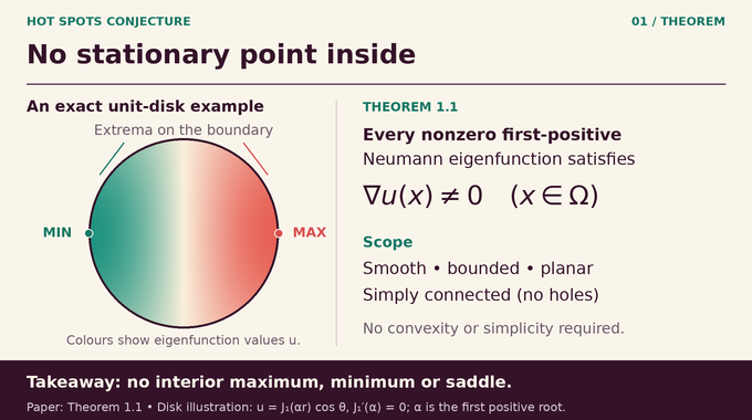
Theorem 1.1 concerns a nonempty bounded open region with boundary and no holes. Write for its first positive Neumann eigenvalue and for the associated real eigenspace. For every nonzero , it proves:
| Question | Verified Scope |
|---|---|
| Geometry | Nonempty, smooth, bounded, simply connected planar domain |
| Eigenfunctions | Every nonzero member of the first positive Neumann eigenspace |
| Conclusion | No interior critical points; all global extrema occur only on the boundary |
| Extra shape assumptions | No convexity, reflection symmetry or simple-eigenvalue assumption |
| Excluded scope | Arbitrary domains with holes, higher dimensions and nonsmooth boundaries |
Consequently, every interior value lies strictly between the boundary minimum and maximum. Excluding interior critical points of eigenfunctions is stronger than locating global extrema: a saddle has zero gradient without being hottest or coldest. The theorem covers every eigenfunction in the eigenspace, rather than selecting one favorable representative.
“Strict” is a pointwise statement, not a uniform temperature gap. Interior points can approach a boundary extremum, so their values can approach its value by continuity. Likewise, a gradient that never vanishes inside need not have a positive lower bound throughout the open domain. The theorem excludes zeros without asserting either quantitative bound.
2. Why Does the Heat Equation Lead to Neumann Eigenfunctions?
An insulated boundary permits no normal heat flux. Its spectral modes satisfy the Neumann Laplacian problem:
Here is the Laplacian, the outward unit normal, and the normal derivative. Constants have eigenvalue zero. Expanding heat flow in Neumann eigenfunctions gives exponentially decaying nonconstant modes. When the initial temperature has a nonzero projection onto the first positive eigenspace, that projection supplies the leading long-time deviation from the conserved average.
Some sources call this a “second Neumann eigenfunction” because they count the constant mode first. This paper counts positive eigenvalues only. Its variational definition is:
The space consists of square-integrable functions with square-integrable weak first derivatives. The mean-zero constraint removes constants. This quotient measures spatial variation relative to amplitude. It identifies a slow heat mode, rather than a particular temperature experiment or a measured cooling rate.
3. Why Earlier Hot Spots Proofs Could Not Settle the General Planar Case
Earlier results exploited geometry. Jerison and Nadirashvili handled convex planar domains with two perpendicular reflection symmetries. Other work treated antisymmetric eigenfunctions, lip domains and nearly circular convex shapes. Triangle results, including Judge and Mondal’s work with its erratum, address domains with corners. The paper’s introduction distinguishes those results from its smooth-domain theorem.
Topology also obstructs unrestricted claims. Burdzy and Werner constructed a counterexample with two holes. Subsequent work produced examples with both extrema strictly inside, eventually with just one hole. Simply connectedness therefore excludes known failure mechanisms.
The remaining difficulty is directional. On an arbitrary smooth outline, neither Cartesian derivative must keep one sign. The Neumann condition says something different: the gradient is tangent to the boundary. Scalar multiplication preserves that tangency, even around an indentation. This proof develops that observation without assuming a globally preferred direction. For wider context on how topology enters mathematical claims, see our Hilbert–Smith explainer.
4. The Spectral Foundations: Eigenvalue Separation and Multiplicity
Lemma 2.1 first establishes , where is the lowest Dirichlet eigenvalue. Dirichlet data prescribe a function’s boundary value, while Neumann data prescribe its normal derivative. The strict separation later prevents an unwanted component from surviving in an equality case. The proof uses plane waves and finite dimensionality to rule out equality.
Next, the positive and negative nodal sets of every nonzero are connected. If three sign components existed, restrictions to two components could form a mean-zero Rayleigh minimizer vanishing on the third. Analyticity would force that eigenfunction to vanish everywhere, a contradiction.
On the boundary circle, four cyclically alternating strict signs would require positive and negative connecting paths to intersect. That planar obstruction, combined with a positive weighted boundary mean-zero condition, proves Proposition 2.5: . This known multiplicity bound is a crucial constraint, not an assumption of eigenvalue simplicity. It should not be confused with unrelated many-body gaps discussed in our spectral-gap explainer.
5. How the Proof Transforms the Domain Into a Disk
Lemma 2.2 supplies a conformal bijection extending to a smooth diffeomorphism of closures, with nonvanishing derivative. Here is the open unit disk. This regularity matters: boundary gradients and tangent data must remain controlled. Our Brennan conjecture article provides related background on conformal derivatives.
The geometry reappears as a potential measure . Conformal invariance of the planar Dirichlet integral transfers the spectral gap into:
The subscript zero means zero boundary trace. This “subcritical” inequality makes the Green operator a contraction on the weighted square-integrable space. Its resolvent therefore exists and can be expanded as a convergent Neumann series. Mapping to a disk simplifies the boundary without discarding the domain’s influence: that influence sits in the potential.
A useful distinction is that the proof extends the original Cartesian components of the physical gradient. It does not silently replace them by the gradient of the pulled-back eigenfunction, which would introduce derivatives of the conformal map. Keeping the physical components fixed allows the final kernel evaluation to recover the actual gradient at the suspected critical point.
6. Rohleder’s Variational Principle: Controlling Tangent Vector Fields
For a vector field with square-integrable first derivatives and tangent boundary trace, define as the integral of squared divergence plus squared scalar curl. Proposition 3.1 gives the first anchor:
Equality holds exactly when for some . This is Rohleder’s variational principle, with its equality case derived in the paper. It turns the spectral problem into a test for recognizing eigenfunction gradients.
The proof decomposes into a gradient and a rotated gradient. Simple connectivity removes a residual field that is tangent, divergence-free and curl-free. The two surviving components are orthogonal. The ordinary gradient is controlled by , while the rotated gradient is controlled by the larger . Equality therefore eliminates the rotated component.
This precise equality characterization makes zero excess energy informative. A field attaining equality must come from the original eigenspace. That structural use of energy differs from the nonlinear PDE mechanism in our Lane–Emden explainer.
The zero field is allowed in this equality space. What ultimately matters is producing independent nonzero fields from a single assumed critical point. Thus the argument needs both parts of the variational statement: nonnegativity makes a zero sum decisive, and the equality case converts each vanished energy into a genuine eigenfunction.
7. Building the Green Kernels and the Boundary Energy
On the disk, the Dirichlet Green function represents interior forcing, while the Poisson kernel extends boundary data harmonically. Adding the potential through the convergent resolvent produces two positive kernels with complementary roles:
| Object | Role |
|---|---|
| Carries boundary data to the interior evaluation point . | |
| Measures interaction between distinct boundary points, including the potential correction. | |
| Measures excess vector energy for the extension of tangent boundary data ; always nonnegative. |
Specifically, extend each fixed Cartesian component of by the transformed Helmholtz equation, then return to the physical domain to obtain . Set . Its nullspace consists exactly of boundary data whose extensions are gradients from .
For an eigenfunction , let on . The Neumann condition makes tangent and gives . Positivity here concerns an entire quadratic form. It does not say that every term in a boundary integral is positive. Keeping those meanings separate is essential, as in other operator arguments such as our Crouzeix inequality explainer.
8. The Multiplier Identity: The Proof’s First Decisive Step
Multiply by any real Lipschitz boundary function . The field remains tangent. Proposition 4.4 expresses its excess energy entirely through differences of multiplier values:
Both integrals use circle arclength, whose total mass is . To obtain the identity, compare the bilinear energy of and with the energy of . Nonnegativity and imply . Subtraction cancels the boundary-curvature terms, leaving the squared multiplier difference.
The singularity is manageable: Lipschitz differences cancel the inverse-square singular part of . The sign is harder. Gradients at two boundary points can point in opposing directions, so can be negative. Choosing one arbitrary multiplier does not solve the problem. The proof needs a coordinated family whose squared differences neutralize the kernel.
9. Reciprocal Green Kernels and Conditional Negative Semidefiniteness
Theorem 5.1 supplies that family indirectly. For each interior , define:
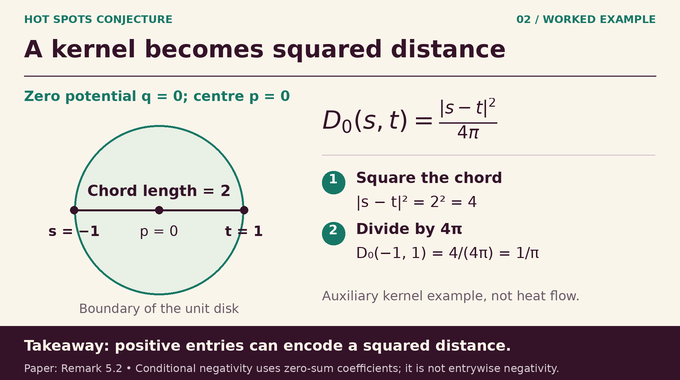
The theorem proves conditional negative semidefiniteness: whenever finitely many real coefficients satisfy , one has . The zero-sum restriction is essential. This is a squared-distance condition, not a claim that the positive off-diagonal entries are negative.
The innovation is proving it for a singular Green kernel after a nonnegative subcritical potential is added. The paper first builds bounded regularizations whose entrywise reciprocal matrices have at most one positive eigenvalue. “Reciprocal” means replacing each entry by its reciprocal, never taking a matrix inverse.
A finite algebraic lemma preserves this property under rank-one updates along columns of the current kernel matrix. Positive quadrature nodes then add successive contributions to the Green resolvent. The proof passes through quadrature refinement, removal of regularization, a radial boundary limit, and finally removal of a compact-support cutoff. That order avoids assuming individual Poisson kernels belong to the weighted square-integrable space when they may not.
Concretely, a node updates entries by with . The coefficient sums repeated visits to that node in the resolvent expansion. After suitable diagonal rescaling, the new reciprocal matrix is a positive rank-one matrix minus a positive semidefinite matrix. It therefore still has at most one positive eigenvalue. This is a preservation theorem for the entire finite configuration, rather than an estimate of isolated entries.
Adjoining to finitely many boundary points gives a bordered reciprocal matrix. Its one-positive-eigenvalue bound forces nonpositivity on a particular hyperplane. Rescaling coefficients by converts that hyperplane into the required zero-sum condition. This bridges finite matrix algebra and boundary analysis.
A checked example makes the distance interpretation concrete. With zero potential and , Remark 5.2 gives . Opposite unit-circle points have squared chord length four, so their kernel value is . This auxiliary example illustrates Theorem 5.1, not a zero-potential Neumann eigenfunction experiment.
10. How Hilbert-Space Multipliers Eliminate Every Interior Critical Point
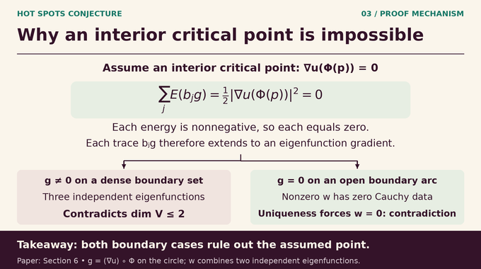
Schoenberg’s correspondence realizes as the squared distance between and in a real Hilbert space. The resulting map is injective and Lipschitz. Its coordinates are admissible scalar multipliers. Summing their energy identities cancels and factors the remaining double integral into a squared interior evaluation:
Dominated convergence justifies the potentially infinite sum. If were critical, the right side would be zero. Each energy is nonnegative, so every one vanishes. Each multiplied trace must therefore extend to another eigenfunction gradient.
If the set where is dense on the circle, injectivity prevents its Hilbert-space image from lying in an affine line. Two coordinates then make , and independent. That requires three independent eigenfunctions, contradicting .
If that set is not dense, vanishes on an open boundary arc. A nonconstant multiplier produces a second independent eigenfunction. Their traces are constant on the arc, so a nonzero linear combination has both zero value and zero normal derivative there. Zero extension across that arc and interior analyticity force it to vanish throughout the domain. Independence gives the contradiction. Neither case allows an interior critical point.
The two cases also explain why a boundary arc with zero gradient cannot simply be ignored. Dense nonzero boundary data support the dimension argument. An actual open gap instead supplies the paired boundary conditions needed for uniqueness. The proof closes both possibilities without imposing a special boundary sign pattern.
11. What the Strict Hot Spots Proof Establishes and Its Limits
This hot spots conjecture proof establishes the strict hot spots conjecture and excludes saddles as well as interior global extrema, without convexity, symmetry or eigenvalue simplicity. Its reciprocal-kernel theorem also applies to any bounded nonnegative disk potential satisfying the subcritical inequality, independently of conformal geometry.
The main theorem concerns smooth, bounded, simply connected planar domains. It does not automatically cover corners, holes or higher dimensions. Smoothness is a stated hypothesis, even though boundary analyticity is unnecessary. Assumption sensitivity also matters in our Shub entropy conjecture analysis.
The heat-flow interpretation also concerns a leading asymptotic mode. An arbitrary initial temperature may have no component in this eigenspace, and transient heat patterns combine many modes. The theorem supplies no numerical convergence time, solver benchmark or computational speedup. Its achievement is an exact qualitative constraint on the specified eigenfunctions.
The paper is dated September 24, while OpenAI’s release announcement is dated October 6, 2026. The family 369 scope note describes the same full interior and boundary-extrema target, including multiplicity. However, the linked comparator statement ends with a sorry placeholder. That file specifies a target rather than completing its proof. The separately supplied Lean proof entry could not be retrieved for inspection here, and no Lean build was run. Accordingly, this article verifies the mathematical exposition against the PDF without claiming independent verification of the implementation. Our Lean proof explainer discusses the broader formal-proof context.
The enduring insight of the Hot Spots Conjecture result is how boundary information rules out an unseen stationary point: nonnegative energies, engineered through reciprocal kernels, would create more eigenfunction gradients than planar topology permits. Follow Binary Verse AI for evidence-led explanations that make mathematical mechanisms and their limits readable.
Has OpenAI proved the hot spots conjecture?
OpenAI’s September 2026 paper proves the strict hot spots conjecture for every nonempty smooth, bounded, simply connected planar domain. Every nonzero eigenfunction of the first positive Neumann eigenvalue has no interior critical point, so its maximum and minimum occur exclusively on the boundary. The theorem does not establish this conclusion for arbitrary domains in all dimensions.
What is the mathematical formula for the hot spots conjecture?
For a first-positive Neumann eigenfunction , the eigenvalue equation is in , with on its boundary. The paper proves the stronger condition for every interior point , which implies strict inequalities between every interior value and the boundary extrema.
Why is excluding interior critical points stronger than locating maxima on the boundary?
A critical point occurs wherever . It may be a maximum, minimum or saddle point. The classical hot spots conclusion concerns global extrema, whereas OpenAI’s theorem excludes all three types of interior critical points, including saddles that would not violate the weaker statement.
Why does simply connectedness matter in this proof?
Simply connectedness supports the disk conformal parametrization and the planar topological arguments used in the proof. Earlier counterexamples showed that the general hot spots conjecture can fail on domains with holes, including a single hole. Thus the theorem’s topological restriction is mathematically substantive.
Does the proof require a convex domain or a simple Neumann eigenvalue?
No. The theorem assumes neither convexity nor symmetry, and it applies even when the first positive Neumann eigenvalue is multiple. The proof establishes that the corresponding real eigenspace has dimension at most two and uses this fact in the final contradiction.
How does OpenAI’s proof rule out an interior critical point?
The argument constructs a nonnegative energy whose zero-energy fields are precisely first-positive eigenfunction gradients. A reciprocal Green-kernel theorem supplies Hilbert-space multipliers. At an assumed interior critical point, these force additional zero-energy gradients. Depending on the boundary-gradient support, this contradicts either the eigenspace dimension bound or boundary uniqueness.