
A matrix can have only zero eigenvalues and still amplify a vector by a factor of two. That small surprise explains why Crouzeix’s conjecture matters: eigenvalues do not tell the whole story of nonnormal matrices. The right geometric object is their numerical range.
OpenAI’s September 26, 2026 direct proof establishes the sharp constant 2 for polynomial evaluation with arbitrary finite-dimensional matrix coefficients. Earlier scalar proofs had already appeared. The advance here is the complete inequality, which remains valid as both matrix dimensions and polynomial degree vary independently.
Its mechanism connects convex geometry, Fourier coefficients, and a positive block matrix. Following that connection reveals what was proved, why multiplication order matters, and where the exact constant comes from.
Table of Contents
1. What Is Crouzeix’s Conjecture? The Original Numerical-Range Problem
The numerical range of a matrix collects its quadratic-form values on unit vectors:
Here the star denotes conjugate transpose, and vector norms are Euclidean. Matrix norms are induced operator norms, measuring maximum vector amplification. The numerical range is compact, convex, and contains every eigenvalue. The scalar conjecture asks for
| Feature | Precise Scope |
|---|---|
| Manuscript | OpenAI, September 26, 2026; direct finite-dimensional proof. |
| Main constant | Exactly 2, uniformly over matrix sizes and polynomial degree. |
| Coefficients | Arbitrary square complex matrices, including scalars. |
| Matrix assumptions | No normality or nonempty-interior assumption. |
| Evidence | Proof manuscript and repository formalization documentation; no independent Lean rebuild here. |
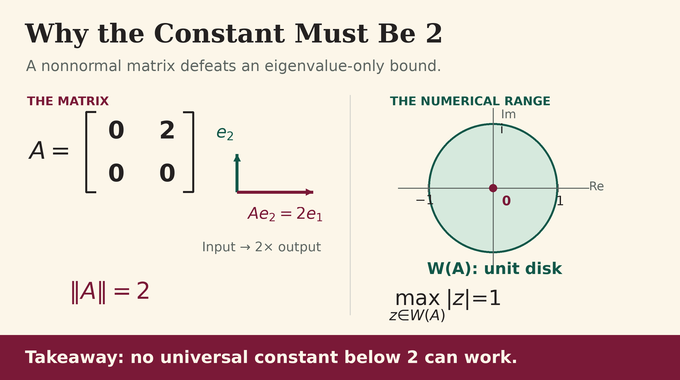
For a normal matrix, which commutes with its adjoint, the spectral theorem already controls polynomial evaluation using eigenvalues. Contrast the nonnormal matrix
Its square vanishes, so both eigenvalues are zero. Yet its norm is 2. With , the maximum over eigenvalues is zero, making an eigenvalue-only bound impossible. Its numerical range is instead the closed unit disk.
2. Why the Sharp Constant 2 Was So Difficult to Prove
Crouzeix posed the scalar question in 2004 and established a universal complete bound of 11.08 in 2007. The Crouzeix–Palencia theorem reduced it to in 2017. That was already dimension independent, but still above the conjectured optimum.
Scalar proofs appeared in 2026, including Shanmu Jin’s preprint and Emiel Lorist and Felix Schwenninger’s argument. Thus “Crouzeix conjecture solved” needs a scope qualification: OpenAI’s direct paper tackles the complete extension. Scalar functional-calculus arguments can use commutation identities that fail when coefficients become matrices.
Complete constant-two results also existed for restricted base dimensions. The direct paper cites the two-dimensional case and a 2026 result for dimensions at most three. Neither restriction settles the theorem for arbitrary base matrices. The issue was retaining the optimal bound while removing both dimension restrictions.
As in our Naimark problem coverage, identifying the contribution requires separating an earlier resolution from a new proof or stronger statement.
3. What OpenAI’s Complete Crouzeix Theorem Actually Proves
Theorem 1.1 allows any positive base dimension , any positive coefficient dimension , and any nonnegative degree . Write , with . Its tensor evaluation is
The tensor product places the base matrix first and acts on a space of dimension . For matrix-valued polynomials, the complete Crouzeix conjecture becomes
Setting recovers the scalar statement. Completeness requires exactly the same constant for every coefficient size. In spectral-set terminology, this is the complete 2-spectral set bound, expressed here for polynomials.
For developers, it supplies a worst-case certificate for polynomial matrix transformations. A scalar polynomial approximation error can be bounded over the numerical range before evaluating the matrix. It does not demonstrate faster training or a numerical-software speedup, a distinction also central to our log-concave sampling explainer.
For example, a residual represented by a scalar polynomial satisfies . This follows immediately from the theorem and the operator-norm definition. Finding a small maximum remains an approximation problem; the theorem does not choose the polynomial for you.
OpenAI’s release announcement attributes the collection to an internal frontier model. The family 325 scope documentation reports formalization covering the finite-dimensional bound, sharpness, and broader operator results. Those broader results exceed this paper’s stated theorem. This article does not independently rebuild Lean, run its comparator, or establish journal peer review. Our Fermat formalization guide explains why statement scope and verification remain distinct.
4. Mapping the Numerical Range Onto a Smooth Convex Domain
First enclose the numerical range strictly inside a bounded convex domain with regular real-analytic boundary. This temporary smoothness permits convergent boundary expansions. An exterior conformal map sends the exterior unit disk onto the exterior of the domain and continues across its boundary.
On the unit circle, write . This nonzero vector points outward, although it is not generally a unit normal. Convexity supplies the supporting-line inequality
Every interior point lies on the inward side of the tangent line. The conjugation turns complex multiplication into the appropriate real inner product. Our Brennan conjecture explainer introduces related conformal-map language, although the estimate here concerns matrix evaluation.
5. How Faber Polynomials Turn Boundary Geometry Into Coefficients
This map parametrizes the exterior, rather than sending the domain itself into a disk. That choice produces Laurent expansions at infinity. The analytically continued collar around the unit circle later ensures genuine convergence, instead of leaving the proof dependent on formal series manipulations.
Theorem 2.1 defines its polynomial basis through an expansion at infinity:
If , then , and has degree with leading coefficient . These are Faber polynomials for that exterior coordinate.
For positive k, their crucial feature appears after returning to the boundary:
A nonconstant basis polynomial has one positive Fourier mode and only negative modes besides it. The mixed coefficients describe that correction. They come from subtracting the circle’s Cauchy kernel from the mapped kernel. Analytic continuation makes their double series absolutely and uniformly convergent on the boundary, justifying the integrations that follow.
The correction in the next section has expansion . The first index labels the input Faber polynomial and the second labels its negative output frequency. The argument does not assume that swapping those indices leaves the coefficients unchanged.
6. The Positive Kernel That Controls the Negative Fourier Modes
Define the mixed correction and its real kernel by
For distinct unit-circle points, the real part of the circle term contributes one after doubling. Consequently by the supporting-line inequality. The apparent diagonal singularity cancels in the correction, so continuity preserves positivity there.
Use normalized angular measure . Every mixed term has nonzero frequency in each variable, giving
These two identities make the associated integral operator an contraction: Jensen’s inequality controls each averaged value, and the other marginal controls its integral. Both normalizations matter. A one-sided averaging argument would leave the total energy uncontrolled.
More explicitly, . Applied to , integration cancels the constant and conjugate correction terms. The surviving mixed term produces precisely the negative-frequency part required by the Faber expansion.
7. The Coefficient Norm Estimate: Where the Factor 2 First Appears
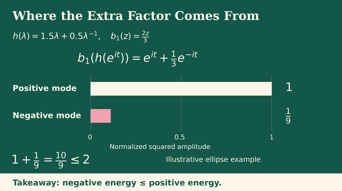
Write . The Hilbert–Schmidt norm is the square root of the sum of squared entry magnitudes. Unlike the operator norm, it gives a Hilbert-space coefficient geometry.
The boundary expansion separates into a constant, positive frequencies, and negative frequencies. Parseval’s identity makes their squared energies add. The contraction bounds negative energy by positive energy, proving Proposition 2.2:
Here the boundary norm integrates squared Hilbert–Schmidt norms against normalized angular measure. Orthogonality prevents cancellation between different frequencies, the same basic principle used in Fourier analysis of wave estimates.
| Coefficient | Boundary Upper Weight | Dual Weight |
|---|---|---|
| Constant | 1 | 1 |
| Nonconstant | 2 |
The lower bound simply retains the constant and positive energies, which are already nonnegative. For the upper bound, the negative part contributes at most one additional copy of the positive energy. No pointwise comparison between individual Fourier coefficients is required.
Only nonconstant coefficients can generate negative-frequency energy. Their weight doubles; the constant’s does not. Keeping that asymmetry is essential to the final comparison.
8. The Resolvent and the Positivity Behind OpenAI’s Proof
Now reintroduce the matrix through its resolvent:
The scalar expansion becomes . Strict spectral separation gives geometric coefficient decay and uniform convergence. Its average is the identity.
More decisively, , where the symbol means positive semidefinite. To see why, set . Direct multiplication gives
Testing the right side against a unit vector produces twice the supporting-line expression with . That point belongs to the numerical range, so the result is nonnegative. Invertibility of the resolvent denominator transfers positivity back. The boundary geometry has become a matrix inequality.
9. Why Singular Vectors and Both Products FG and GF Are Essential
Normalize a polynomial so its boundary operator norm is at most one, and put . The zero case is immediate. Otherwise choose unit singular vectors satisfying
Explicitly, and , with of size . The vectors are standard coefficient-space basis vectors. Unit normalization gives , while preserving all correlations between the two tensor factors.
Encode their tensor coordinates by matrices , and define , , , and . We use D and E for the paper’s diagonal fields P and Q. Subscripts denote their negative Fourier coefficients. Set .
The coefficient pairing gives . Taking shows . Evaluation preserves multiplication in order, yielding two different tests:
Left and right multiplication by the boundary contraction F each decrease Hilbert–Schmidt norm. Applying both coefficient estimates therefore bounds both diagonal functionals. Duality reverses the coefficient weights:
A concrete warning is supplied by matrix units: has one nonzero entry, equal to one, in row and column . Then , whereas . Even constant matrix-valued polynomials can therefore give different ordered products. Completeness requires a proof that respects this elementary difference.
Concretely, test with entrywise conjugate coefficients, halving each nonconstant one, then pass through finite truncations. Interchanging FG and GF would erase one required estimate. Matrix coefficients do not grant that shortcut.
10. The Final Positive Block Argument: Deriving the Exact Bound 2
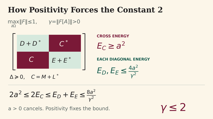
Compress the positive resolvent field with the combined matrix of singular-vector coordinates:
Let denote the integrated squared Hilbert–Schmidt norms of its two diagonal fields and its lower cross field. Parseval gives and : the constant doubles before squaring, while each nonconstant mode appears with its adjoint.
For the cross field, . Its energy is therefore
Nothing discards the constant coefficient. Finally set . Both and are positive, so their product has nonnegative trace. Expanding that trace and integrating gives . Thus
The constant follows from matching coefficient weights with positive block geometry. It is an exact universal bound, rather than a numerical fit.
11. Extending the Proof to Every Numerical Range, and Showing 2 Is Optimal
Smoothness was scaffolding. Lemma 4.1 constructs analytic convex outer domains around every nonempty compact convex set, including a point or segment. Their maximum distance from the set tends to zero. Applying the domain bound and uniform continuity of the fixed polynomial makes the boundary maxima converge to the maximum on the numerical range.
The construction combines finitely many supporting directions using exponentials of affine functions. Including both coordinate axes ensures boundedness and a positive-definite Hessian. A regular level curve then supplies the analytic boundary. This explains why the approximation remains available even when the original set has no interior.
Sharpness returns to the displayed nilpotent example with . For a unit vector, , with equality when both coordinates equal . Every phase and radius up to one occurs. Meanwhile , so its norm is exactly 2. Consequently
Crouzeix’s conjecture reaches its precise endpoint: constant 2, arbitrary finite coefficient size, and no missing degenerate numerical ranges. For applications, the next task is obtaining useful numerical-range enclosures and approximation bounds. For readers, the reusable insight is how geometry becomes positivity, then a norm estimate. Continue with Binary Verse AI’s guide to evaluating AI mathematics and follow our research explainers for proofs unpacked with their assumptions intact.
What is Crouzeix’s conjecture?
Crouzeix’s conjecture states that for every square complex matrix and scalar polynomial , . Here is the numerical range and the norm is the Euclidean operator norm. OpenAI’s direct paper proves the stronger matrix-valued polynomial inequality.
Was Crouzeix’s conjecture already solved before OpenAI’s proof?
Yes. Scalar proofs appeared in 2026, including work by Shanmu Jin and by Emiel Lorist and Felix Schwenninger. OpenAI’s September 26 direct paper addresses the complete inequality, allowing arbitrary finite-dimensional matrix coefficients with the same constant 2. This distinguishes the earlier scalar resolution from the complete result.
What makes the complete Crouzeix inequality different from the original conjecture?
The scalar inequality corresponds to coefficient dimension . The complete inequality requires constant 2 for every matrix-coefficient dimension , independently of the base matrix size and polynomial degree. Proving the scalar case alone does not automatically establish this uniform matrix-valued extension.
Why does OpenAI’s proof use both FG and GF?
Matrix coefficients generally do not commute, so and cannot be interchanged. Testing both products separately gives bounds for the two diagonal coefficient functionals associated with the right and left singular vectors. Both estimates are needed in the final positive block comparison.
How do Faber polynomials help establish the sharp constant 2?
They express polynomial boundary values as a constant term, positive Fourier modes, and controlled negative modes. A nonnegative kernel with both marginal integrals equal to one bounds the negative-frequency energy. The resulting coefficient weights combine with resolvent positivity and the two ordered product tests to produce the sharp bound.
Why can’t the constant in Crouzeix’s inequality be smaller than 2?
Take and . The matrix has operator norm 2, while its numerical range is the closed unit disk, where the maximum of is 1. Equality holds, excluding every smaller universal constant.
Does OpenAI’s direct proof cover matrices with numerical ranges that are points or line segments?
Yes. The proof first works with analytic convex domains, then encloses any compact convex numerical range in such domains with distance tending to zero. Uniform continuity passes the polynomial bound to the limiting numerical range, including points and line segments.