
After three Thorp shuffles, every card in an eight-card deck has exactly the right chance of occupying every position. Yet almost nine-tenths of all deck orders remain impossible. Each card looks innocent. The correlations give the game away.
The Thorp shuffle mixing time asks how quickly the entire deck becomes approximately uniform. OpenAI’s September 26, 2026 paper proves that, for cards, the answer has order . Its explicit upper construction uses complete shuffles, while counting possible outcomes forces a lower bound of . The achievement is matching growth rates for the full permutation, rather than merely scattering individual cards.
Table of Contents
1. What OpenAI Proved About Thorp Shuffle Mixing Time
In Optimal-order mixing of the Thorp shuffle, let denote one shuffle’s probability law and the uniform law on all permutations. Theorem 1.1 states:
The star denotes convolution, meaning composition of independent random permutations. Total variation is the largest probability discrepancy over events. Consequently, closeness controls every test of the final deck, including tests involving many cards simultaneously. The switch-chain mixing problem uses the same distributional criterion for graphs.
1.1. Thorp Shuffle Mixing Time: Key Facts
| Research Detail | Verified Scope |
|---|---|
| Deck size | labeled cards. |
| One time step | One complete physical shuffle, using fair bits. |
| Mixing criterion | Total-variation distance at most . |
| Upper conclusion | Distance after shuffles tends to zero as . |
| Necessary time | At least shuffles. |
| Not determined here | Sharp leading constant and cutoff for this model. |
OpenAI’s mathematics release announcement attributes the collection to an internal frontier model. The family 238 formalization scope explicitly reports the main optimal-order theorem, alongside separately scoped supporting results. This article explains the supplied manuscript and that documentation, without independently rebuilding Lean. Our Fermat formalization explainer explains why discovery and machine checking are different contributions.
2. How Does the Thorp Shuffle Actually Work?
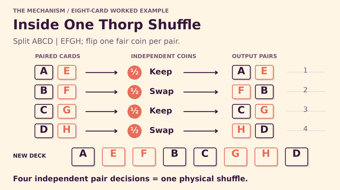
Split eight cards into equal halves: A, B, C, D and E, F, G, H. Pair corresponding positions: A with E, B with F, C with G, D with H. Flip four independent fair coins. Each coin decides which member of its pair comes first. Concatenate the four resulting pairs.
That example produces A, E, F, B, C, G, H, D. A complete physical shuffle uses four coin flips here, generally . Repeat the same operation on the newly ordered deck, with fresh independent coins.
This differs from ordinary riffle shuffling, whose random cut and interleaving follow another probability model. A familiar bound for riffle shuffles cannot be imported into the Thorp model simply because both interleave cards. The transition rule determines the theorem.
3. Why Randomizing One Card Does Not Randomize the Deck
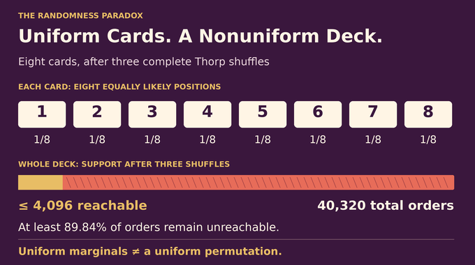
Track one card through three shuffles of eight cards. Each shuffle refreshes one binary coordinate of its position. After three refreshes, its three-bit position is uniform over eight possibilities. This holds separately for every card.
The whole deck has a stricter requirement. Three shuffles consume twelve random bits, so they can produce at most deck orders. There are possible permutations. Thus at least 36,224 orders are unreachable, despite perfectly uniform single-card positions.
This is a distinction between marginals and their joint distribution. Cards share switches, and permutations forbid collisions. The resulting dependencies survive tests that examine only one card. Trace reconstruction offers a related lesson about information hidden in joint positional structure, although its deletion model is different.
4. The Original Problem and Why Earlier Proofs Fell Short
Edward Thorp introduced the model in his 1973 study of nonrandom shuffling and Faro. Its elementary rule left a difficult quantitative question: how long do dependencies across the complete permutation persist?
The manuscript traces successive improvements from Morris’s bound to Montenegro and Tetali’s . Morris then developed entropy methods, first obtaining for every even deck size and later for powers of two. These are upper guarantees, rather than measurements of typical simulations.
4.1. How the Proven Upper Bounds Changed
| Method Or Authors | Upper-Bound Order |
|---|---|
| Morris: evolving sets and chameleon process | for dyadic decks. |
| Montenegro–Tetali: refined analysis | for dyadic decks. |
| Morris: entropy methods | for even decks; later for dyadic decks. |
| This manuscript | for dyadic decks. |
Entropy measures departure from a reference distribution. Its usefulness across probability and information theory also appears in our Courtade–Kumar explainer, but the shuffle requires its own contraction argument.
Previous work also controlled large selections of cards without settling the complete permutation at logarithmic time. The new Thorp shuffle proof connects a conditional-flow estimate to a separate representation-theoretic argument. Sampling one valid object and sampling the right ensemble remain different achievements, as in counting perfect matchings.
5. Why the Mixing Time Cannot Beat 2d Minus a Constant
Every physical shuffle uses independent bits. After shuffles there are only possible coin strings. Different strings might coincide, so this is an upper bound on the number of reachable permutations, not an assumption that all outputs differ.
Let be that reachable set. The shuffle assigns probability one to , while uniform randomness assigns at most its size divided by . Therefore:
Distance at most one-quarter requires at least three-quarters of the permutation space to be reachable. Taking binary logarithms gives the necessary bound:
The paper obtains this order using elementary factorial inequalities. It counts available randomness, whereas logarithmic-space derandomization asks when algorithms can eliminate random choices. Having enough bits is necessary here, but does not establish that the shuffle uses them effectively.
6. Turning the Thorp Shuffle Into a Binary Hypercube
Write positions as binary strings in , the set of length- bit vectors with addition modulo two. For eight cards these are 000 through 111. Paired positions differ in the first bit.
A physical shuffle first independently swaps or fixes each pair, then rotates the coordinates. Its position rule is:
Here contains the remaining bits and is that pair’s fair bit. Addition in the last coordinate is modulo two.
Undo the known rotation when describing the evolving deck. In this moving frame, successive updates become switches along successive cube coordinates. One full coordinate sweep takes physical shuffles. For example, the first-coordinate edge from 000 to 100 and the second-coordinate edge from 000 to 010 are different matching edges. A layer uses only one direction at a time, so each position belongs to exactly one active pair. This bookkeeping matters: the theorem counts physical shuffles, not sweeps. For eight cards, toggling the first, second, then third coordinate is three layers, not one operation. At a full sweep’s end, the accumulated rotation returns to its starting frame.
7. Conditional Probability Flow: Tracking the Unexposed Cards
Choose an ordered random list of labels independently of the shuffle. Reveal their complete paths one at a time. After exposing cards, let be the free positions at time , with constant size . The next, tagged card has conditional probabilities .
Subtract the uniform distribution on those free positions:
The indicator equals one on free positions and zero elsewhere. Thus sums to zero. It records excesses and deficits relative to the desired conditional distribution.
With two free endpoints, the switch coin is unexposed, so both probabilities average. With one free endpoint, an observed card’s path determines the switch, and the tagged-card probability follows the remaining route. Revealing feasible paths fixes exactly the coins those paths visited. Other coins remain independent and fair. This fact justifies conditioning on trajectories without quietly inventing independence between all remaining card positions.
8. The One-Sweep Energy Identity That Makes the Proof Work
Let average values across coordinate- pairs. The actual centered flow equals that ideal averaging plus conditional mean-zero noise from switches with one free endpoint. Noise here describes uncertainty revealed by observed paths, rather than extra randomness added to the shuffle.
Define , the expected sum of squared deviations. Let be the expected sum of over free positions whose partner in the next active direction is occupied by an exposed card. Lemma 3.2 gives, for :
This equality retains exactly one sweep of noise. Averaging through all coordinates erases the old mean-zero vector. Cross terms vanish because later noise has conditional mean zero. A noise contribution from layers ago spreads over disjoint subcubes, leaving the factor in squared energy.
The result is sharper than repeatedly bounding every update separately: it identifies precisely which recent obstructions still matter. The weights are not arbitrary discount factors fitted to data. They follow from how averaging spreads an edge-supported perturbation through the remaining coordinates. The proof therefore needs the prescribed coordinate order, rather than silently replacing it with randomly chosen directions.
9. How Independent Cube Halves Force the Energy to Contract
Before a coordinate becomes active again, the intervening directions never cross its two opposite cube halves. Conditional on the earlier exposed history, the future switch arrays inside those halves are independent.
This separates a flow value in one half from the availability of its partner in the opposite half. It does not assert independence between flow and availability within the same half. That distinction is where a tempting shortcut would fail.
Averaging over random input lists leaves the free set uniformly distributed among subsets of its size. When at least positions remain, concentration makes very sparse halves rare. Combining this with the energy identity gives, for :
The first term decays geometrically, while the second bounds exceptional configurations. Sequentially comparing each tagged card with a uniform free position converts energy into total variation. After shuffles, the ordered positions of a uniformly chosen list of cards have average error . “Average” matters: this intermediate guarantee is not stated uniformly over every prescribed list.
10. From Nearly Randomized Cards to the Entire Permutation
Knowing seven-eighths of the deck approximately does not automatically control the hidden eighth. Partition labels into eight equal blocks, each containing cards. The averaged estimate guarantees a partition whose eight complementary marginals have small total error.
For each omitted block, permutations agreeing outside it form a coset of the subgroup that rearranges only that block. Remove cosets carrying excessive probability, doing all eight removals together. Conditioning on the retained set produces one nearby law, , satisfying every coset cap simultaneously. Separate trimming for each marginal would not provide this common law.
Representation theory now decomposes permutation dependence into matrix-valued components. These are Fourier matrices on the symmetric group, rather than the scalar frequency coefficients familiar from the discrete Fourier transform.
The hook-length formula controls representation dimensions through Young diagrams. Restricting to the eight block subgroups exposes a small-dimensional factor. Controlling a vector’s orbit span, even when representations occur repeatedly, yields:
More concretely, within each tensor component the eight factor dimensions multiply to at most , so at least one is at most . The orbit-span estimate then produces a squared-norm exponent of , hence after taking square roots.
Here is irreducible, its dimension, the operator norm measures maximum amplification, and is an absolute constant.
11. Completing the Proof: Why Eight Blocks of 200d Shuffles Suffice
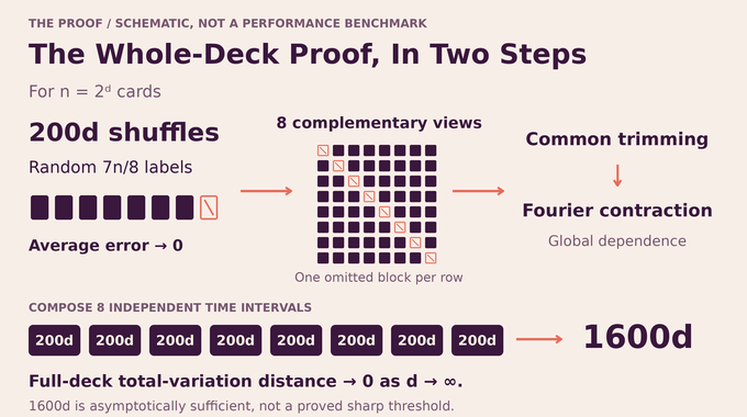
Compose eight independent intervals, each lasting physical shuffles. Convolution multiplies their Fourier matrices. The resulting dimension decay makes the sum of all nontrivial, nonsign contributions vanish, using the reciprocal-dimension estimate proved earlier. Specifically, eight factors and squared norms supply the exponent in representation dimension. The remaining reciprocal-cube sum tends to zero. These eight time intervals are distinct from the eight label blocks used to establish each interval’s Fourier estimate.
Parity needs separate treatment because the sign representation has dimension one. In a positive-time original interval, flipping one final switch coin reverses permutation parity. Even and odd outcomes therefore balance exactly. Trimming introduces only a vanishing bias, which remains harmless after eight factors.
Replacing each trimmed interval with its original law costs at most its total-variation difference. Eight replacements still cost a vanishing amount. This completes the full-permutation comparison after shuffles, from every deterministic starting deck.
Once the full law is close, every fixed selection of cards is close too, because applying a deterministic observation cannot increase total variation. That stronger conclusion arrives at the end, rather than being assumed in the averaged intermediate estimate.
For developers, the theorem implies approximately uniform permutations using independent fair bits. It supplies no competitive implementation benchmark. As in log-concave sampling, an asymptotic guarantee must be read alongside the resource being counted. The paper’s dyadic proof does not establish the same bound for 52 or 100 cards, determine the sharp leading constant, or settle cutoff, an abrupt mixing transition. Nor does distributional mixing alone establish an efficient keyed cipher’s security, a distinction relevant to our AI cryptography coverage.
Thorp shuffle mixing time now has its optimal growth order. The lasting insight is how local conditional averaging, carefully preserved independence, and global algebra together control correlations invisible to single-card tests. Explore Binary Verse AI’s linked proof explainers to keep building that distinction between what a theorem proves and what an application still needs.
What is the mixing time of the Thorp shuffle?
For cards, the paper proves mixing time , using total-variation distance one-quarter as its threshold. This concerns the entire permutation approaching uniform, rather than merely individual card positions.
Why is the result called optimal-order mixing?
The necessary lower bound is , and the sufficient upper bound is . Both grow linearly with , although their constants differ. Optimal order does not mean an exact leading constant.
Does OpenAI’s proof establish that exactly 1600d shuffles are necessary?
No. The theorem shows that the distance from uniform after shuffles tends to zero as . It does not assert that this many shuffles are necessary or give that numerical guarantee for every finite dimension. The sharp constant and cutoff remain separate questions.
Why can every card be uniformly distributed while the deck is not?
Uniform individual positions do not eliminate correlations between cards. After three shuffles of eight cards, every card is individually uniform, yet at most 4,096 of the 40,320 complete deck orders are reachable.
Is the Thorp shuffle the same as ordinary riffle shuffling?
No. The Thorp model pairs corresponding cards from two equal halves and independently chooses the order inside each pair. Ordinary riffle shuffling uses a different transition law. Its familiar seven-shuffle result should not be applied to this model.
Does the theorem apply to a standard 52-card deck or a 100-card deck?
Not directly. This optimal-order theorem concerns deck sizes . The manuscript does not establish the same quantitative result for arbitrary even deck sizes, including 52 and 100.
Does this proof immediately produce a practical secure block cipher?
No. It establishes full-permutation mixing under independent fair switch bits and has cryptographic relevance. It does not itself prove the security or practicality of a concrete efficient keyed cipher.