

A noisy qubit can lose an excitation, gain one from its surroundings, and still carry a precisely calculable amount of classical information. OpenAI’s September 24, 2026 paper proves that the generalized amplitude damping channel has classical capacity equal to its one-shot Holevo capacity for every allowed damping strength and thermal occupation. Two equally probable pure states achieve the optimum. Entangling signals across channel uses cannot improve the rate.
The difficult part was ruling out those entangled encodings, rather than finding attractive single-qubit signals. The proof supplies an entropy inequality that survives thermal excitation and remains valid across arbitrarily long input blocks. It turns a potentially enormous optimization into a maximum over one real variable.
Table of Contents
1. What Is the Generalized Amplitude Damping Channel?
A density matrix records a qubit’s populations and coherence. Write its diagonal entries as and , with off-diagonal entries and . The paper takes as the excited state. Its stationary excited-state population is , a convention worth checking before comparing formulas across sources.
The transformation replaces the diagonal populations by and and multiplies both coherences by the same square-root factor. A valid input satisfies . Coherence describes the off-diagonal information that distinguishes a superposition from an ordinary population mixture. At stationarity, the population stays fixed, while coherence still decays whenever damping is positive.
| Quantity | Meaning |
|---|---|
| Damping strength | |
| Stationary excited-state population | |
| Output excited-state population | |
| Coherence decay | |
| Capacity | Unassisted classical bits per independent use |
Thermal noise permits upward and downward transitions. The generalized amplitude damping Kraus operators make this explicit. With , they are , , , and . The channel maps to , where the star denotes the adjoint. Their adjoint products sum to the identity.
These equations specify a memoryless model. They do not establish that every laboratory device has exactly this noise. That distinction matters throughout quantum computing and artificial intelligence.
2. Why Was Its Classical Capacity So Difficult to Determine?
Holevo information subtracts average individual-output entropy from the entropy of the average output. Maximizing that difference gives the one-shot quantity . “One-shot” here describes the ensemble optimization, not a promise that separately measuring each qubit achieves that rate.
The operational question asks how many classical message bits can be transmitted per use with error tending to zero as codes grow longer. The sender has no preshared entanglement with the receiver and receives no feedback. Entanglement among the sender’s input qubits is nevertheless permitted. Those are different resources, and the theorem optimizes over the latter.
Earlier work characterized the generalized channel’s one-use optimum. The Khatri–Sharma–Wilde study compared it with upper bounds on unrestricted capacity. In general, quantum channel additivity fails: a better ensemble can emerge when several uses are optimized together. Capacity therefore requires regularization, taking the supremum of per-use Holevo information over every block length.
Ordinary damping admits a pure output, enabling an earlier additivity theorem. At positive damping and interior thermal occupation, every output is full rank, so that criterion fails. The unital midpoint and entanglement-breaking regimes had separate solutions. OpenAI’s argument covers the whole parameter square. It addresses information transmission, distinct from the ground-state entanglement question in the 2D area law.
The paper credits Tang, Zhu, Bai, and Wang for the triangular inequality and the pure-output channel results. Its extension preserves the useful entropy contribution when both thermal transitions are present. This attribution identifies the new step without treating the entire proof apparatus as newly invented.
3. OpenAI’s Exact Capacity Theorem: From Many Qubits to One Variable
Theorem 1.1 of the capacity and entropy inequalities paper gives the following generalized amplitude damping capacity formula. Abbreviate the channel by and define as the scalar objective:
Here is the input excited-state population. The binary entropy is , with . The determinant entropy function is for . Both use natural logarithms. Dividing by converts nats to bits.
Throughout the proof, denotes von Neumann entropy in nats. For a normalized state, its eigenvalues form a probability distribution. Entropy is their Shannon entropy. The notation also applies to positive matrices that are not normalized, which is why the block inequalities explicitly divide Gram matrices by their masses.
More strongly, for every integer . The tensor product denotes independent channel actions, while the input ensemble remains unrestricted. This is the step that removes regularization.
4. Why Two Opposite-Phase Pure States Achieve the Optimum
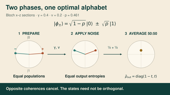
Choose the following signals with equal probability:
Their populations agree, but their coherences have opposite signs. After damping, both outputs have excited population and coherence magnitude . Their spectra, and hence their entropies, coincide.
Averaging the outputs cancels the opposite coherences. The mean becomes diagonal, with entropy . Each signal output has entropy . Their Holevo difference is exactly . Maximizing the population therefore constructs an attaining ensemble, without searching over arbitrary collections of qubit states.
The two states need not be orthogonal. This is a communication ensemble, not a computational-basis alphabet. The coding theorem allows the receiver to decode long output blocks collectively.
At the midpoint population, the signals are the familiar plus and minus superpositions. Away from that population, their inner product is . Choosing a different population changes both their distinguishability and the entropy created by noise. The scalar maximization balances those effects, rather than automatically choosing the most widely separated inputs.
5. Output Entropy, Determinants, and the Crucial Convexity Property
For a two-dimensional state, trace one and the determinant determine both eigenvalues. Taking the determinant of either phase-pair output gives . Completing the square yields:
Define . Lemma 4.1 proves that this output entropy is convex in population. One cannot infer that simply because is convex: composing functions requires additional conditions.
The proof writes as the Euclidean norm of an affine two-component vector. It is convex. The separately established function is nondecreasing and convex on . Their composition proves the required convexity, including endpoints. This lets conditional populations recombine without losing the entropy bound.
6. The First Proof Ingredient: A Triangular Block Entropy Inequality
Theorem 2.1 starts with equal-shaped rectangular matrices and a block factor . Their squared Hilbert–Schmidt masses are , , and , summing to one:
The entropy of is at least the weighted entropies of the three normalized block Gram matrices, plus . Terms with zero weight are omitted. The extra term measures the entropy forced by the block arrangement.
For intuition, replace the blocks by the scalars , , and . The resulting Gram matrix has trace one and determinant , so its entropy is exactly . The theorem says that allowing internal matrix structure cannot erase this contribution after the internal entropies are accounted for. It is an inequality for noncommuting matrices, not an assumption that all blocks share eigenvectors.
The proof converts equal-trace entropy differences into convergent log-determinant integrals. A jointly convex Schur-complement expression then permits averaging over coordinate signs, removing off-diagonal structure in the comparison matrices. Concavity and homogeneity of the scalar deficit combine the resulting coordinate bounds. Here is Shannon entropy in nats.
Zero padding extends the argument to rectangular blocks without changing nonzero eigenvalues. This matters because output dimension need not equal the number of Kraus operators. As in Crouzeix’s matrix inequality, keeping block structure intact carries information that a scalar shortcut can discard.
7. The Thermal Extension: Two Factorizations with One Entropy Bound
Thermal excitation fills the zero block that made the previous estimate usable. Theorem 3.1 handles rectangular matrices with . Define and . Then:
The four coefficients are nonnegative, sum to one, and satisfy , with . Set , , and .
Keeping row sums and coherence fixed leaves the line . Its endpoints respectively have and . Each admits a zero-block Gram factorization, after a row swap where necessary. Both yield exactly the same scalar contribution .
The original state is a convex mixture of those endpoint states. Entropy concavity preserves the common scalar term and combines their branch weights, giving:
The proof separately handles . It assumes neither orthogonal branches nor commuting Gram matrices. That flexibility makes the thermal extension useful for entangled inputs.
8. The Site-by-Site Argument for Entangled Multi-Qubit Inputs
Split any pure input into its first-qubit branches. The normalized branch vectors can overlap and remain entangled across later sites:
Apply an arbitrary finite-dimensional channel to those branches. Placing its Kraus images in columns constructs and retains the cross operator . Lemma 4.2 then gives:
For repeated damping, choose the partner as the remaining channel uses. Iterate the lemma. At each site, convexity of combines conditional populations into the original marginal population . Writing for the full output, Proposition 4.3 establishes:
For example, equally weighted branches with later-site populations 0.2 and 0.8 give marginal population 0.5. Convexity says the average branch entropy contribution is at least the contribution at 0.5. This is precisely the direction needed for a lower bound. Repeating that averaging across sites avoids assuming the input itself factorizes.
Entropy concavity extends this to mixed inputs. Crucially, the bound retains every population, instead of replacing all terms by a universal minimum. The related entropy photon-number inequality also links sharp entropy control to communication, but concerns a different, bosonic setting.
9. Closing the Proof: Why Entangled Encoding Cannot Increase Capacity
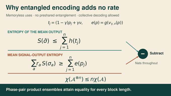
Section 5 now sandwiches the two terms in Holevo information. For any ensemble of block inputs, the preceding result lower-bounds average signal-output entropy by , where populations now refer to the ensemble mean. Convexity justifies this additional averaging.
Meanwhile, entropy of the mean output is no larger than entropy of its computational-basis diagonal. Classical subadditivity bounds that diagonal entropy by . Subtraction leaves at most one scalar optimum per site.
Products of the phase pair attain equality: every individual output and the mean output factorize, so their entropies add. Entangled encoding offers no higher rate. The resemblance to the Courtade–Kumar information problem is conceptual: proving a simple construction optimal requires controlling all competing constructions.
This remains an asymptotic reliable-transmission statement. It supplies neither a finite-length error guarantee nor an implementation of an efficient collective decoder.
10. Additivity with Arbitrary Partner Channels
Corollary 1.2 permits any finite-dimensional completely positive trace-preserving partner , even with different input and output dimensions. It proves:
The branch outputs form a partner-channel ensemble with the correct mean marginal. Subtracting entropy bounds leaves the damping objective plus at most the partner’s Holevo capacity. Product ensembles supply the matching lower bound.
Minimum output entropy is nats, attained at population . Applying one-shot partner additivity against every tensor power and regularizing proves capacity additivity. The partner retains its own regularization: may differ from .
These are three particular additivity results, not a restoration of additivity for all quantum channels. Nor does classical capacity specify the rate for transmitting unknown quantum states. Changing the communication resource or allowing a channel with memory changes the problem being solved.
11. Exact Limits, Worked Example, and What the Formalization Covers
| Parameters | Exact Consequence |
|---|---|
| Ordinary amplitude damping | |
| Identity channel: 1 bit per use | |
| Fixed thermal output: 0 bits per use | |
| Capacity unchanged by exchanging basis states |
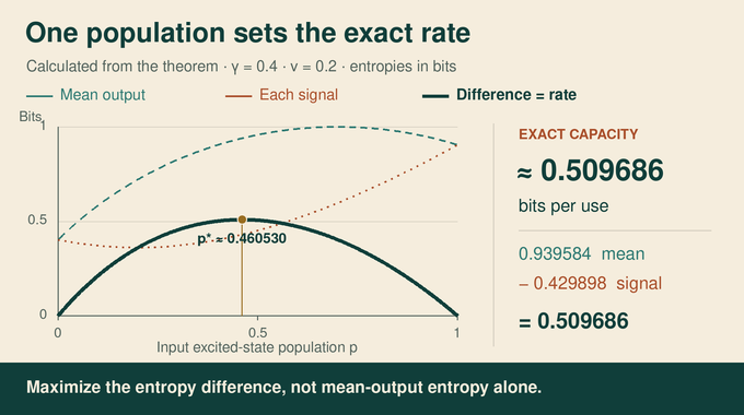
For a worked example, set and . Numerical maximization gives , output population , and determinant . Mean-output entropy is approximately 0.939584 bits, while individual-output entropy is 0.429898 bits. Subtracting gives 0.509686 bits per use. These are calculations from the theorem, not measured hardware performance.
The optimizer was checked against a dense population grid. Its population differs from the entropy-minimizing population 0.2 because maximizing communication also rewards entropy of the mean output. Minimizing noise on each signal alone does not maximize their Holevo difference. This is why retaining the population dependence throughout the proof pays off.
At zero thermal occupation, the determinant reduces to , recovering ordinary damping. At the unital midpoint, symmetry and concavity put a maximizer at . Complete damping instead makes every signal output identical, so no information remains, even if the fixed output has nonzero entropy. The identity endpoint preserves a full classical bit. Thermal reflection exchanges the basis states and replaces the optimizing population by .
The family 276 Lean scope document covers exact capacity, repeated-use Holevo additivity, and attainment by maximizing phase-pair product ensembles. It explicitly excludes arbitrary-partner additivity and separate-measurement decoding. That is documented scope, not a report of a fresh Lean build here. Our Fermat formalization explainer explains why matching formal and informal statements matters.
OpenAI released this work within its AI mathematics research collection. The cited manuscript is a public preprint. Its mathematical proofs and documented formalization are distinct from independent expert review or a communication experiment. For developers, the immediate benefit is a compact reference calculation against which to compare simulated signaling strategies under this noise model.
The generalized amplitude damping channel now has a remarkably economical capacity description: optimize one population, prepare a phase pair, and keep the decoding distinction clear. Follow Binary Verse AI for source-led explanations that connect theorem statements, proof mechanisms, and what researchers can actually use.
What is the difference between amplitude damping and generalized amplitude damping?
Ordinary amplitude damping models relaxation toward the ground state. Generalized amplitude damping also permits thermal excitation, with a nonzero stationary excited-state population. In the paper’s convention, ordinary damping is the special case .
What do γ and ν represent?
In the paper, is the damping strength and is the stationary excited-state population, both in . The case gives ordinary amplitude damping, while is the unital midpoint.
What is the classical capacity of a generalized amplitude damping channel?
OpenAI’s Theorem 1.1 proves that its unassisted classical capacity equals its one-shot Holevo capacity for every allowed parameter pair. Both are given by the one-variable maximum stated in the article. The entropy functions use natural logarithms, and division by gives bits per use.
Why do two pure quantum states achieve the optimal capacity?
The attaining ensemble uses two equally probable pure states with opposite phases and a maximizing excited-state population. Their output entropies agree, while their opposite coherences cancel in the average output. Their Holevo information therefore equals the exact scalar optimum.
Can entangled inputs increase the classical capacity of this channel?
No, within the paper’s memoryless, unassisted model. Arbitrary entangled inputs across repeated uses cannot exceed the rate achieved by independent phase-pair signals. Collective decoding remains allowed. Product encoding does not imply that separately measuring each output achieves capacity.
What role does minimum output entropy play in the proof?
The entropy argument bounds output entropy for entangled inputs while retaining each site’s excited-state population. That stronger bound enables the capacity proof. The paper also obtains in nats and proves minimum-output-entropy additivity with every finite-dimensional partner channel.
Does Lean verify every result in OpenAI’s paper?
No. The documented formalization covers exact capacity, repeated-use Holevo additivity, and attainment by maximizing phase-pair product ensembles. Arbitrary-partner additivity and decoding by separate measurements are explicitly outside that scope. This article does not report an independent rerun of the Lean proof.