

A computer can draw a turbulent-looking standard map in seconds. Proving that its chaos occupies positive area, rather than an intricate set of area zero, is a different problem entirely. OpenAI’s September 23, 2026 paper proves that standard map chaos has this stronger, measurable form for every sufficiently large positive parameter. Its result concerns the exact deterministic sine map, with no added noise or perturbation.
The proof connects exponential instability to entropy, then rules out a subtle escape route: repeated cancellations that could erase strong local expansion over long times.
Table of Contents
1. What OpenAI’s Proof Establishes About Standard Map Chaos
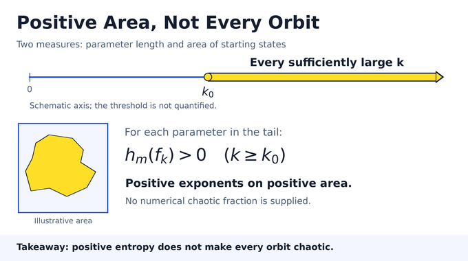
Theorem 1.1 of the research paper states that a positive threshold exists beyond which normalized area has positive metric entropy:
Here, is the map, is area normalized to total mass one, and is entropy relative to that measure. Equivalently, a positive-area set of initial states has a positive largest Lyapunov exponent.
| Question | Precise Answer |
|---|---|
| Source | OpenAI manuscript, September 23, 2026; Theorem 1.1. |
| System | Exact smooth, deterministic sine map on the two-dimensional torus. |
| Measure | Normalized invariant Lebesgue area. |
| Parameter Scope | Every , for some positive threshold. |
| Quantitative Limits | No numerical threshold, chaotic-area fraction, or uniform positive entropy bound. |
The quantifier “every” makes this stronger than locating favorable parameters scattered through a large-parameter range. It still leaves room for regular trajectories elsewhere.
OpenAI’s release announcement attributes the collection to an internal frontier model. The family 146 formalization scope reports coverage of the entropy theorem, positive exponents, and the hyperbolic-component corollary. This article explains the released argument and reported formalization scope, without an independent Lean rebuild. Discovery and formal verification remain distinct tasks, as our Fermat formalization explainer illustrates.
2. The Standard Sine Map: The Equation Behind the Proof
The Chirikov standard map acts on the two-dimensional torus: a unit square whose opposite edges are identified. Coordinates wrap modulo one. Writing the next coordinates with primes, the paper’s map is
Read this as a kick followed by a drift. First increase the second coordinate by the sine term. Then add that updated coordinate to the first. The amplitude controls the kick’s strength.
Put . Differentiating gives
Its determinant is . The map is invertible, so this establishes area preservation. Stretching in one direction must be balanced by contraction in another.
For large amplitudes, the cosine term often produces strong derivative growth. Near its zeros, that simple picture weakens. Even away from those locations, expanding directions can change between steps. Large entries alone do not settle long-term instability.
3. Sinai’s Positive Entropy Conjecture: The Original Mathematical Problem
In the formulation addressed here, Sinai’s positive entropy conjecture asks for positive metric entropy on a positive-measure set of parameters. Two different measures appear: length along the parameter axis and area among initial conditions at each parameter.
The theorem supplies an entire positive parameter tail, . Each parameter in that tail has its own positive-area set of exponentially unstable states. Neither the area nor the entropy is given a uniform positive lower bound.
A residual set of parameters, meaning a countable intersection of open dense sets, need not have positive length. Thus even a topologically abundant collection of favorable parameters cannot substitute for the conjecture’s measure requirement. The full-tail conclusion avoids that distinction entirely.
Numerical trajectories suggested extensive chaos long before this proof. But any finite computation observes only finitely many steps and starting points. It cannot alone establish an infinite-time exponent on positive area.
This is a question about discrete conservative dynamics. It differs from counting isolated periodic motions in continuous planar systems, the subject of our Hilbert’s 16th problem explainer. Both illustrate why a convincing picture of trajectories still needs a theorem specifying exactly what is being measured.
4. Why Earlier Standard Map Results Could Not Resolve the Conjecture
Earlier work exposed substantial structure. Hyperbolic basic sets support uniformly expanding and contracting directions, but may occupy zero area. Transitive invariant sets of full Hausdorff dimension also fall short: dimension two does not force positive two-dimensional Lebesgue measure.
Positive topological entropy answers another question. It detects orbit complexity available somewhere in the system, whereas positive standard map entropy here must hold for the particular invariant area measure. A measure maximizing entropy need not equal area.
| Question | Precise Answer |
|---|---|
| Hyperbolic Set | Its area may be zero. |
| Full Dimension | Full Hausdorff dimension need not mean positive area. |
| Topological Entropy | Complexity need not be seen by invariant area. |
| Metric Entropy | Specifies both dynamics and invariant measure. |
Noise, coupling, or smooth perturbations can produce useful hyperbolicity while changing the system or probability law. They do not automatically establish the theorem for this exact sine family.
Likewise, “mixing” in a randomized sampler, such as the switch chain, concerns convergence of distributions. The standard-map theorem does not provide a global mixing-time bound. Readers approaching this through log-concave sampling should keep that distinction between stochastic guarantees and deterministic instability in view.
5. Lyapunov Exponents And Kolmogorov–Sinai Entropy
The standard map Lyapunov exponent measures asymptotic derivative growth. For almost every state , the largest exponent is
The derivative of the nth iterate multiplies derivatives along the orbit. Logarithms convert exponential growth into a rate per iteration. the limit concerns infinitesimal perturbations, not indefinite exponential separation of two points across a compact torus.
Area preservation pairs the two exponents as and , with the largest nonnegative. Pesin’s entropy formula then gives
The map is smooth, the torus compact, and area an absolutely continuous invariant probability measure. These properties supply the required integrability and regularity. Ergodicity is not assumed.
Kolmogorov–Sinai entropy describes the rate at which orbit observations generate information, optimized over finite measurable partitions. Positive exponents on positive area make the integral positive. The word “entropy” does not make this the same quantity as quantum-state entropy in the entropy photon-number inequality; the measure and mathematical definition matter.
6. Transfer Matrices: Measuring Growth Along Standard Map Orbits
Write the state at integer time as , and set . Since modulo one, a fixed coordinate change produces the recurrence
Locally chosen real lifts allow differentiation. A small displacement obeys a linear recurrence with matrix
Thus carries to . Its determinant is one. Products transport perturbations between times.
Set , a convenient one-step norm bound. The paper records growth and expected shortfall as
Expectation averages over uniformly distributed initial states. Growth lies between zero and elapsed time, so the shortfall lies between zero and one. Natural logarithms still define entropy and Lyapunov exponents.
7. Why Rapid Expansion Can Cancel: The First Key Estimate
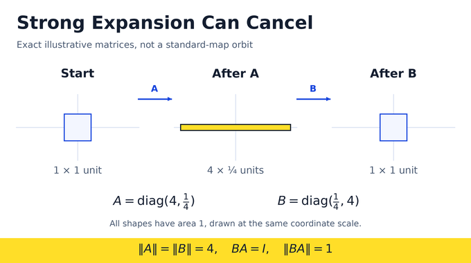
Consider the exact toy matrices and . Each has norm four and determinant one, yet . Strong expansion in separate pieces can disappear upon composition.
1. Start
Square: side 1 unit.
2. Apply The Stretch
Rectangle: 4 by ¼ units.
3. Apply Its Inverse
Square: side 1 unit again.
Theorem 3.1 handles the relevant orbit-dependent version. If two length-n transfers from a common center grow nearly at the maximal logarithmic rate, while the full transfer between their outer endpoints grows very little, the event has area probability at most . The positive constants are uniform for sufficiently large parameters.
Here probability means the area of initial states producing that event. No random kicks have been inserted.
Why should cancellation be rare? Singular-direction geometry produces a solution of the linearized recurrence that is appreciable near the center but tiny at both distant endpoints. That simultaneous boundary behavior imposes restrictive conditions along both outward paths. Counting those conditions, rather than merely counting large derivatives, drives the argument.
More precisely, both outward logarithmic norms must be at least , while the concatenated norm’s logarithm is at most . The small positive constant is chosen by the proof, rather than fitted to simulations.
The estimate does not outlaw all cancellation. It controls a precise extreme event strongly enough to constrain how growth deficits accumulate.
8. Matched Expansion Scales And The Local Scarcity Argument
Follow the orbit outward from the central site in both time directions. “Good” indices combine near-maximal derivative growth with rapid decay of the specially chosen small-endpoint solution. A shortfall-counting lemma shows that sufficiently small total deficits leave many such indices.
An auxiliary solution starts with values zero and one. On either outward path, the conserved Wronskian identity is
This prevents the two solutions from collapsing together. The proof matches indices on opposite paths where their derivative expansion scales are comparable, then rescales the varying initial coordinate.
The central compatibility condition becomes an approximate relation between a cubic polynomial and two reciprocal-cosine expressions. The phases are nearly affine after rescaling. If successful configurations occupied too much local length, a positive-measure limit would force an analytic identity that the proof excludes.
The delicate cases are essential: the reciprocal terms might nearly cancel, or one phase slope might approach zero. Separate derivative estimates rule out those degeneracies uniformly. The resulting local scarcity, combined across many matched tests with controlled distortion, yields exponential decay. It does not assume those tests are independent.
9. Fast Bridges: Controlling Distant Orbit Segments Without Independence
Theorem 5.1 supplies the second quantitative ingredient. A “fast bridge” is a long orbit segment whose transfer matrix has sufficiently strong growth. The theorem bounds weighted observations near its opposite ends by a controlled product-type estimate plus an exponentially small correction.
The observations are bounded Lipschitz functions of finitely many local shortfalls. One is a nonnegative weight; the other tests whether a shortfall-related quantity exceeds a fixed positive threshold. Constants and minimum lengths can depend on those observation bounds.
The product-type bound retains a dependence on the frequency of the far-end event, with its threshold relaxed by a factor of two. That detail lets it control rare events weighted by another local deficit, instead of treating distant windows as independent random samples.
Finite Dirichlet boundary problems provide the geometry. Fixing a distant coordinate constructs contracting graphs through eligible states. Forward and backward graph families are transverse. Along one family, the distant observation changes very little; moving across the other family controls how much area the weight contributes.
Bounded slice Jacobians justify these changes of variables. The resulting estimate applies without presuming statistical independence or global mixing, including at arbitrarily large eligible bridge lengths.
This is a useful methodological lesson for developers studying deterministic data: stationarity does not imply independence. Uniform marginal coordinates at each time do not make distant observations unrelated.
10. Dyadic Scales And The Geometry Of Limiting Growth
Suppose, for contradiction, that arbitrarily large parameters have zero largest exponent almost everywhere. At each such parameter, increasing orbit length makes the expected shortfall tend to one. Conversely, at each fixed finite length, increasing the parameter makes the shortfall tend to zero.
These limits point in opposite directions. Cancellation scarcity controls how much shortfall can increase when length doubles. The proof chooses a slowly increasing starting length and the first dyadic length where a small deficit threshold is crossed. It normalizes by that terminal shortfall.
Rescaled growth distances enter a compact space of semimetric arrays: tables of growth between pairs of rescaled times. A semimetric permits distinct times to have zero distance. Constant-speed arrays must be tracked separately because weighted mass can approach them in the limit.
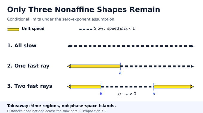
No Exterior Fast Ray
One Exterior Fast Ray
Two Exterior Fast Rays
For the nonconstant configurations, the bridge estimate, cancellation bound, and four-point comparison leave three possibilities: entirely slow behavior, one exterior unit-speed ray, or two exterior unit-speed rays surrounding a positive-length slow interval. “Speed” means normalized logarithmic derivative growth, not a particle’s physical velocity. Distances need not add across the slow region.
11. The Final Capped-Deficit Contradiction
The final observable caps the shortfall: it grows with a small slope near zero and equals one on uniformly slow intervals. Compare its value on a whole interval with the average on its two halves. Summing these differences across dyadic scales telescopes.
The starting contribution disappears after normalization, while the terminal contribution remains positive. The limiting measure separates into backward dilates of a terminal measure and a translation- and dilation-invariant remainder.
The terminal contribution is strictly smaller than that required positive balance. If its measure is nonzero, a slow interval remains detectable at arbitrarily fine scales. The invariant remainder contributes at most zero. For two-ray configurations, averaging compares fine-scale occupancy of the slow interval against the smaller capped loss on long crossing intervals.
The affine speeds require three treatments. The cap is flat on slow speeds, the bridge estimate removes intermediate speeds, and cancellation truncation controls the unit-speed case. Ordinary convergence away from these arrays would otherwise miss potentially decisive weighted mass.
The two contributions cannot supply the positive telescoping balance. The zero-exponent sequence is impossible.
Theorem 1.1 follows. Corollary 1.2 then yields a positive-area invariant ergodic hyperbolic component. It splits into finitely many cyclic pieces, each Bernoulli under the corresponding iterate. This does not prove ergodicity of the entire torus, almost-everywhere chaos, an explicit threshold, or a practical simulation speedup.
For AI readers, this is research-level reasoning rather than an LLM math benchmark score. Standard map chaos now has a positive-area theorem in the released proof. Follow Binary Verse AI’s research explainers to understand the mechanisms, assumptions, and remaining questions behind AI-assisted mathematics.
What does positive entropy mean in the standard map?
Positive metric entropy means measurable dynamical complexity relative to the standard map’s invariant area measure. For this smooth area-preserving map, Pesin’s formula makes it equivalent to a positive largest Lyapunov exponent on a set of initial conditions with positive area.
What is Kolmogorov–Sinai entropy?
Kolmogorov–Sinai entropy measures the average rate of information generation in a measure-preserving dynamical system. It is defined relative to an invariant probability measure, using measurable partitions. Topological entropy instead describes orbit complexity without fixing that measure.
What exactly did Sinai’s positive entropy conjecture ask?
In the formulation addressed by the paper, it asked whether the standard map has positive metric entropy with respect to area for a positive-measure set of parameters. The released proof establishes the stronger result for every sufficiently large positive parameter.
Does OpenAI’s proof establish chaos for every standard map trajectory?
No. It proves a positive largest Lyapunov exponent on a positive-area set of initial conditions for every sufficiently large positive parameter. It does not show that every trajectory is chaotic or that almost every point has a positive exponent.
Why are Lyapunov exponents important to the proof?
A positive largest Lyapunov exponent describes asymptotic exponential growth of infinitesimal perturbations along an orbit. Pesin’s formula connects these exponents to metric entropy. The proof therefore establishes positive entropy by proving exponential instability on positive area.
Does the proof identify the critical parameter where chaos begins?
No. The theorem establishes a sufficiently large threshold without an explicit numerical value. It does not identify where positive entropy first appears, and its threshold should not be confused with numerical estimates for the destruction of invariant curves.
Does positive metric entropy prove that the entire standard map is ergodic?
No. The paper’s corollary establishes a positive-area invariant ergodic hyperbolic component. That component has a finite cyclic decomposition, with the corresponding iterate Bernoulli on each piece. It does not prove ergodicity or Bernoulli behavior across the entire torus.