
A matrix with rows is a peculiar starting point for avoiding enormous computations. OpenAI’s October 4, 2026 preprint does exactly that: it uses the matrix mathematically, then computes the information it needs without constructing it. The resulting Existential Theory of the Reals proof places exact polynomial feasibility in a fixed level of the counting hierarchy, with the explicit bound for ETR.
The paper also handles one existential real block followed by one universal real block. This is a complexity containment, not a polynomial-time solver. Its central achievement is keeping real solutions, limits, and gigantic algebraic objects under control through a fixed sequence of counting operations.
Table of Contents
1. What Is the Existential Theory of the Reals?
The Existential Theory of the Reals, or ETR, asks whether real numbers exist that satisfy a Boolean combination of polynomial equations and inequalities. “Boolean combination” permits AND, OR, and NOT. Coefficients have finite encodings. All comparisons are exact.
For example, together with is satisfiable: the positive square root works, although no rational number does. Requiring instead gives no real solution. The domain matters, and replacing equality with “close enough” changes the question.
| Manuscript | OpenAI, October 4, 2026 preprint. |
|---|---|
| Existential Bound | and . |
| Two-Block Bound | for an absolute, unspecified integer . |
| Input | Explicit Boolean formula and division-free arithmetic circuits with binary integer constants. |
| Practical Evidence | No implementation benchmark or demonstrated solver speedup is established. |
For developers, this is the mathematical core of continuous constraint feasibility. A numerical optimizer reporting a tiny residual does not automatically certify an exact solution. That distinction is separate from the approximation guarantees discussed in our edit distance analysis.
2. The Original Complexity Barrier: From Tarski to PSPACE
Tarski established decidability for real closed fields: an algorithm can determine the truth of first-order polynomial statements over the reals. Collins’s cylindrical algebraic decomposition supplied a geometric quantifier-elimination method. Decidability, however, leaves enormous room for computational expense.
Canny’s 1988 PSPACE result showed that existential real feasibility can be decided with memory polynomial in the input length. Polynomial space does not imply polynomial time. A procedure may reuse a small workspace across exponentially many steps.
The missing existential theory of reals complexity bound was membership in a more structured hierarchy built from counting. Knowing that ETR lies in PSPACE does not supply that conclusion: the containment runs from each fixed counting level into PSPACE, not automatically back again.
This is a resource-class question, unlike the relative computability studied in our Turing degrees explainer. The present algorithms receive finite bit strings and must account for the cost of manipulating them. An exact real value is not a free, infinitely precise machine register.
Uniformity is essential: one algorithm must work across all valid input sizes, rather than receiving a separately designed solution for each instance. Our generalized star height explainer examines another uniform bound, though its levels measure nested regular-expression operations rather than counting oracles.
3. What OpenAI Proved: ETR Enters the Counting Hierarchy
PP consists of decision problems accepted by polynomial-time probabilistic machines with probability strictly greater than one-half precisely on yes-instances. The margin above one-half may be extremely small. PP therefore expresses majority counting, not the comfortable error guarantee of an ordinary randomized algorithm.
The counting hierarchy starts at . Its next level uses PP machines with an oracle from the preceding level. An oracle is an idealized subroutine answering a specified decision problem. Membership requires a fixed nesting depth, independent of input size.
Appendix A of the research manuscript gives the existential bound:
ETR is a decision problem. The complexity class contains every language polynomial-time many-one reducible to ETR, so the bound transfers to that class. Theorem 1.1 separately places existential universal real sentences with circuit inputs in some fixed level. It does not assign them level 26.
Unlike the query counts in our quantum query complexity explainer, these levels classify nested counting power, rather than accesses to input bits.
For readers following AI mathematical research packages, the useful unit of assessment is the individual theorem and its assumptions. A collection-wide announcement does not establish that every manuscript shares the same verification status, computational model, or kind of advance.
4. How the Proof Converts Arithmetic Circuits Into One Quartic Polynomial
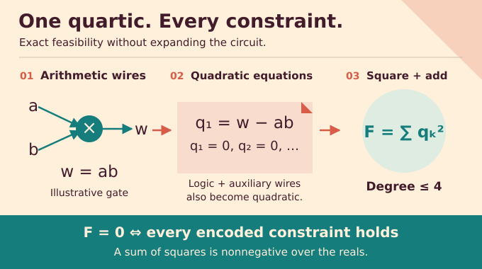
Arithmetic circuit polynomials can have enormous degree despite compact descriptions. Repeated squaring illustrates why: each multiplication gate can double the degree. Expanding the final polynomial would destroy the advantage of the input representation.
Instead, give every gate a real wire variable. A multiplication gate becomes , while addition becomes . Each equation has degree at most two. Boolean variables, constrained by , encode the formula’s logical structure.
Strict positivity also needs an exact witness. For a wire value , the condition is equivalent to the existence of a real satisfying . Additional wires split this product into quadratic equations. The full construction also encodes false atoms and negation, avoiding any assumption that every branch is positive.
If the quadratic left sides are , combine them as:
This nonnegative polynomial has degree at most four. A zero makes every constraint vanish simultaneously. For a quantified sentence, the encoding preserves each fixed parameter : a counterexample to the universal condition exists exactly when the corresponding fiber has a real zero. Compact circuits have become an explicitly listed quartic without expanding their outputs.
5. The Minimization Trick That Turns Real Feasibility Into Algebra
Fix the existential parameter tuple . The proof calls it good when its fiber has no real zero, meaning the universal assertion holds. It studies the objective and minimum:
Here is a penalty parameter, and includes universal variables and auxiliary wires. Sixth powers make the objective coercive: it tends to infinity when the vector escapes to infinity. Its bounded sublevel sets are compact, so a minimum exists.
A zero of the fiber supplies a fixed comparison point. Its penalty vanishes for every , keeping the minimum bounded. Conversely, bounded minima force their minimizing points into a compact set. As the penalty grows, the corresponding values of approach zero. A convergent subsequence then gives an actual zero by continuity.
Thus a good parameter makes the minimum diverge to infinity. Compactness closes the loophole between “arbitrarily small” and “attained.” The existential procedure uses a related coercive deformation, with shifts ensuring a suitable squarefree characteristic polynomial later. These exactness safeguards are part of the proof, rather than numerical convergence assumptions.
Consider . A zero would require both and , which is impossible. Yet choosing and for positive makes the value approach zero as grows. The variables escape while the residual shrinks. The coercive term prevents precisely this behavior when the penalized minimum stays bounded.
6. Why Critical Points Lead to an Exponentially Large Algebra
At a minimizing point, differentiating the objective and dividing by six gives, for each coordinate:
Because the quartic’s derivatives have degree at most three, the pure fifth powers dominate these relations. Modulo the equations, any fifth power can be replaced by lower-degree terms. Repetition leaves a basis of monomials with each coordinate exponent between zero and four.
There are such monomials. The paper proves both spanning and independence, giving a quotient algebra of exactly that dimension. Multiplication by the objective becomes a linear operator on this algebra, with characteristic polynomial:
The symbol denotes the identity matrix and the polynomial’s value variable. Evaluating at a critical point shows that the corresponding objective value is a root. In particular, .
This translates optimization into polynomial algebra but apparently creates an exponential matrix. Our permanent versus determinant explainer examines a different determinant-representation question. Here the obstacle is evaluating information about a structured multiplication operator without writing its entries.
7. How OpenAI Computes Giant Determinants Without Constructing Them
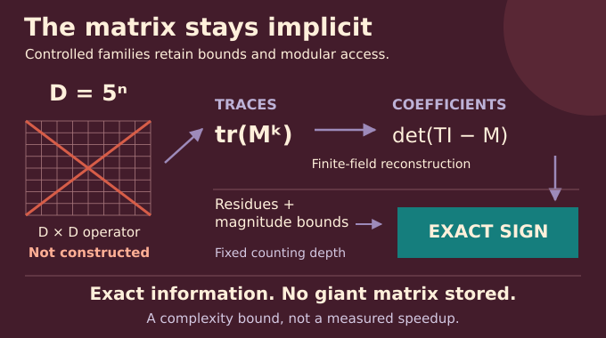
The replacement for a coefficient list is a controlled polynomial family. Each family retains a degree bound, a logarithmic coefficient-norm bound, a prime cutoff, and a uniform procedure for evaluations modulo sufficiently large primes. The bounds themselves have polynomial-length binary encodings.
The trace–residue identity converts the trace of multiplication into a coefficient extraction involving the defining equations and their Jacobian determinant. Traces of powers then determine characteristic coefficients through a formal exponential identity. Over a sufficiently large prime field, all required small denominators are invertible.
Finite-field sums extract indexed coefficients. The algorithm evaluates these sums and products through counting procedures, rather than materializing their exponentially many terms. The Jacobian is only an determinant. The multiplication matrix of dimension remains implicit.
This representation differs from promising that every intermediate has a small arithmetic circuit. The manuscript explicitly supports families without short coefficient lists or circuits. Its closure rules permit a fixed number of constructions, not arbitrary input-dependent nesting. Representation costs are equally central in our exact Fourier transform analysis, although that paper uses a different arithmetic model.
8. Recovering the Signs of Enormous Integers Using Counting
Modular residues reveal an integer only indirectly. One residue cannot tell whether it is positive or negative: both possibilities can leave the same remainder. The proof therefore combines residues across sufficiently many primes with a proven magnitude bound.
Their product exceeds the range needed to distinguish the integer, but that enormous product is never stored. Approximate Chinese-remainder reconstruction instead locates the integer divided by the product, modulo one. Successive powers of two amplify a nonzero value until it falls safely away from the wraparound point.
At the first suitable scale, a controlled approximation lies on different sides of one-half for positive and negative integers. Zero produces no suitable scale. Explicit error margins make the final sign exact despite the approximate intermediate calculation.
Prime products, sums, and quantified index tests each consume bounded counting levels. Crucially, a polynomial-length tuple is treated as one index, so having many coordinates does not create one oracle layer per coordinate. As in our Subset Sum proof explainer, modular information becomes useful only after the argument controls what that information can distinguish.
9. How Short Root Labels Replace Exponentially Long Root Descriptions
Real root isolation presents another representation trap. A polynomial can have exponential degree, making an ordinary full root description too long. Thom-style encodings distinguish roots through the signs of successive derivatives, but recording every derivative sign can also require exponential space in the original input length.
The manuscript compresses those signs into a weighted integer sum. Weights are powers reduced modulo a suitably chosen short prime. Polynomial fingerprinting ensures choices that distinguish all distinct real roots. A prescribed root can therefore be selected using three short integers rather than its entire sign string.
A rational sign approximation, followed by clearing positive denominators, converts that label into a polynomial positivity test. The construction accommodates multiplicities when identifying prescribed roots. The existential decision procedure separately arranges a squarefree polynomial before its determinant-sign reduction.
A label selects one acceptable real root. In a multiplication determinant, nonreal roots occur in conjugate pairs, contributing nonnegative factors. A small integer shift avoids zero factors, allowing a negative determinant to certify the desired real root. This is why compressed labels support exact decisions rather than merely approximate root locations.
Appendix A exploits a simpler task: select some acceptable root, instead of identifying an arbitrary prescribed root. Repeatedly keeping a smallest nonempty derivative-sign class yields a logarithmic-length test list. That refinement helps obtain the explicit existential level without extending the same accounting to both quantifier blocks.
10. The Hardest Step: Handling Existential–Universal Real Sentences
Testing one fiber does not describe a good parameter. The proof builds . Its coefficient of is always one. Thus it never becomes the zero polynomial, even when specializing the parameter changes other coefficients.
Goodness is equivalent to for all sufficiently large . Partitioning parameter space by the actual degree of supplies locally uniform root bounds. Continuity then makes goodness locally constant within each degree piece.
Those pieces need not be closed. Adding a variable equal to the reciprocal of the leading coefficient produces a closed algebraic lift. Inside a compact neighborhood, the good and nongood parts can be separated. Another coercive minimization generates characteristic polynomials whose highest nonzero penalty coefficients vanish at coordinates of a suitable limiting good point.
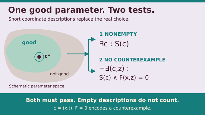
| Nonemptiness | Some real point satisfies the guessed coordinate polynomials and root-label tests. |
|---|---|
| No Counterexample | No point satisfying those same descriptions admits a real zero of the counterexample quartic. |
For intuition, has the good parameter . Finding one counterexample at a different parameter does not refute that sentence. The algorithm must identify a nonempty parameter description whose every selected point survives the counterexample search. This is why another real quantifier block requires additional geometry.
Short guesses select coordinates and labels. Both tests are necessary: an empty description would otherwise pass the no-counterexample test vacuously. Fixed-depth constructions keep the combined decision inside one fixed counting level.
11. What the OpenAI Proof Changes, and What It Does Not
The number 26 is a sufficient upper bound from conservative bookkeeping, not a lower bound or an optimal classification. The two-block result has an unspecified fixed level. Arbitrarily many alternating real quantifier blocks are outside the theorem’s stated scope. No separation between the counting hierarchy and PSPACE is proved.
The source is a released preprint from OpenAI’s mathematics collection. The formalization catalogue checked on October 21, 2026 identifies no paper-specific Lean certificate. That does not establish an error, but publication and machine verification are different evidence, as our Fermat formalization explainer discusses.
For solver developers, the reusable ideas are implicit algebraic representations, exact sign recovery, and compressed witnesses. The paper does not demonstrate faster training, verification software, or optimization workloads. Even an improved asymptotic runtime, such as the result examined in our maximum cardinality matching analysis, requires separate implementation evidence.
The Existential Theory of the Reals result changes how exact continuous feasibility fits into discrete complexity. Its lesson is precise: enormous mathematical objects need not become enormous stored objects. Follow Binary Verse AI for research explainers that trace the mechanism, check the theorem’s scope, and keep practical claims tied to evidence.
What is the existential theory of the reals?
It is the decision problem of determining whether there exist real values satisfying a Boolean combination of polynomial equations and inequalities with finitely encoded coefficients. The comparisons concern exact real values, rather than numerical approximations.
Is ETR the same as the complexity class ∃ℝ?
No. ETR is a decision problem. The complexity class contains all decision problems polynomial-time many-one reducible to ETR.
Is the existential theory of the reals NP-complete?
ETR is NP-hard, but membership in NP is not established. OpenAI’s October 4, 2026 preprint proves the upper bound . This containment does not establish NP-completeness.
Why is membership in the counting hierarchy important?
It provides a more structured complexity upper bound based on a fixed depth of majority-counting operations. It does not establish that the counting hierarchy is strictly smaller than PSPACE.
How can the proof handle exponentially large matrices and polynomials?
It represents controlled polynomial families through short degree and coefficient-size bounds and uniform modular evaluation procedures. A trace–residue identity and finite-field operations recover multiplication-determinant information without constructing the exponentially large matrices.
Does the OpenAI proof handle universal quantifiers over real numbers?
Yes. It handles sentences with one existential real block followed by one universal real block, including arithmetic-circuit polynomial inputs. The block dimensions have no fixed constant bound, but the variable lists are explicitly encoded in the input. The paper does not establish the main theorem for arbitrarily many alternating blocks.
Does OpenAI’s proof make solving real polynomial equations faster?
Not necessarily. Its central contribution is a counting-hierarchy membership theorem. It does not give a polynomial-time algorithm for general ETR or establish a practical solver speedup.