
The De Giorgi conjecture asks whether a phase boundary can bend when the field describing it rises in one fixed direction everywhere. In eight dimensions, OpenAI’s September 26, 2026 preprint proves that it cannot for the scalar cubic Allen–Cahn equation. Every entire solution in the open interval between the two wells with an everywhere positive directional derivative is a hyperbolic-tangent transition across a plane. The proof derives the directional limits that earlier work assumed. Its decisive step takes place one dimension lower, where the paper classifies stable solutions without assuming how quickly their energy grows.
Table of Contents
1. What Does De Giorgi’s Conjecture Say About the Allen–Cahn Equation?
The stationary Allen–Cahn equation describes a field that can interpolate between two preferred values. Here the Laplacian is the sum of the second derivatives in the spatial coordinates. The two wells, and , minimize the quartic potential .
Entire means defined on all of Euclidean space. After rotating coordinates, strict directional monotonicity means at every point. Along each line parallel to the eighth coordinate, the field rises continuously. Its zero crossing, where present, locates the middle of the transition. The conjecture asks whether the whole field depends on one linear coordinate, so that every level in the open range lies on a parallel hyperplane. The September 2026 De Giorgi preprint addresses exactly this question in dimension eight.
| Topic | Finding |
|---|---|
| Equation | Stationary scalar Allen–Cahn with a cubic right-hand side and a quartic double-well potential. |
| Eight-dimensional result | An entire solution strictly between the wells with an everywhere positive directional derivative is a single planar transition. |
| Seven-dimensional result | Every stable entire solution in the closed well interval is a constant well or a planar transition. |
| What changed | The proof derives the directional well limits in dimension eight and the energy-growth bound for stable solutions in dimension seven. |
| Sharp endpoints | Stable nonplanar examples exist in dimension eight. Strictly monotone nonplanar examples exist from dimension nine onward. |
2. What the OpenAI Proof Establishes in Eight Dimensions
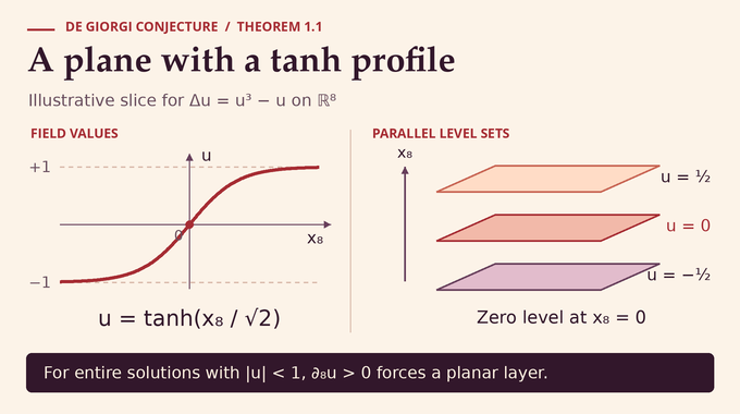
Theorem 1.1 assumes that is twice continuously differentiable on , takes values strictly between the wells, satisfies the equation everywhere, and has . It proves the following formula for a unit vector with and a real offset .
Differentiating the hyperbolic tangent gives
The chain rule gives and . The coordinate is signed distance from the zero plane. For example, choose to be the eighth coordinate direction and set . The field takes the same value at every point with eighth coordinate , namely , regardless of the other seven coordinates.
OpenAI presented the manuscript in its mathematics release announcement. The evidence for this result is the written preprint. Lean coverage for the release is tracked separately in OpenAI’s catalog of formalized main results. For related coverage, see Binary Verse AI’s overview of OpenAI’s mathematics release and its Navier–Stokes and Lean explainer.
3. Why Earlier Proofs Could Not Remove the Extra Assumptions
Ghoussoub and Gui proved the conjecture in dimension two, and Ambrosio and Cabré did so in dimension three. Savin’s flatness theorem reached dimension eight for solutions that approach the lower and upper wells as the monotone coordinate tends to negative and positive infinity, respectively, at each fixed transverse point. In the new proof, the limits initially come from bounded monotonicity alone. That yields two functions of the transverse coordinates, without identifying either function as a constant well.
The dimension cutoff reflects a distinction from the theory of minimal surfaces. Nonflat area-minimizing cones exist in ambient dimension eight, while nonaffine entire minimal graphs first occur in ambient dimension nine. Del Pino, Kowalczyk and Wei’s construction builds nonplanar monotone Allen–Cahn solutions near dilations of such graphs. The resulting examples persist in higher dimensions by adding coordinates on which the field is constant. Dimension eight is therefore the sharp upper endpoint for monotone rigidity. For a different example of a dimension-sensitive PDE result, see the local smoothing conjecture explainer.
4. From Monotonicity to Stability: The First Proof Reduction
Write , where is the eighth coordinate. Differentiating the equation shows that the positive function solves . The stability test asks whether the second variation of the energy is nonnegative for each compactly supported smooth perturbation . Integration by parts using converts that second variation into a weighted square.
Here the second variation has integrand . Bounded monotonicity and elliptic regularity give smooth local limits of vertical translates at both ends. The limits and are independent of . To test their stability in seven dimensions, multiply a transverse test function by a vertical cutoff spread over a length . After dividing by the squared cutoff’s integral, the vertical derivative costs order . Sending to infinity leaves exactly the seven-dimensional stability inequality.
5. The Seven-Dimensional Stability Theorem at the Heart of the Proof
Theorem 1.2 classifies every stable entire solution of the same cubic equation with values in on . The options are the two constant wells or a single planar transition, with an arbitrary orientation in seven dimensions. Stability here allows every compactly supported test. There is no directional monotonicity hypothesis and no prescribed bound on energy growth.
The constant zero solution illustrates what the stability assumption excludes. Its quadratic form has a negative potential term, . For a test function spread over a ball of radius , the gradient term scales like and the negative term like . The latter wins for large , so is negative on those tests. The dimension in Theorem 1.2 is sharp. The preprint cites Pacard and Wei’s stable nonplanar solutions in dimension eight. This leaves room for stable curved interfaces in the very dimension where the monotone theorem forces flatness. For another elliptic problem organized around the distinction between stability and unrestricted solutions, see the Lane–Emden conjecture explainer.
6. How Stable End Profiles Turn Monotone Solutions Into Global Minimizers
The energy over a region combines gradient energy and the potential.
A global minimizer has the least energy in each ball among competitors with its boundary trace. Constant wells have zero energy. For a planar transition, a calibration bounds every competitor’s energy below by the integral of , where . This integral depends only on the boundary trace. The transition attains the bound because .
In a ball, the proof clips an energy-minimizing competitor between and . Taking pointwise minima and maxima preserves the sum of the two energies, and each barrier already minimizes for its own trace. The clipped competitor therefore still minimizes for the original trace. Vertical translates of start above or below that competitor. Sliding the translates back toward zero, strict comparison prevents contact at a nonzero shift. Sliding from both sides identifies the competitor with . A trial field equal to a constant well inside a large ball and joined to in a fixed-width boundary shell then gives the surface-order bound .
7. Finite-Density Rigidity: Defect Estimates, Multiple Sheets, and Stability
Theorem 1.3 gives stable rigidity in dimensions four through seven when normalized energy density stays finite. Here is the ball of radius centered at , is the unit ball volume in one lower dimension, and is the energy per unit area of a planar layer.
Modica’s gradient bound, , gives a nonnegative defect for the inverse profile . For a plane, is signed distance and . Writing , the stability test with amplitude times a cutoff detects a weighted defect term even where the zero set is singular. In the following identity is a compactly supported cutoff and both integrals are over .
If rigidity fails at finite density, the proof reduces to a critical solution of integer density at least two. Away from a sparse exceptional set, its zeros form ordered sheets. A radial Green test gives a lower bound on the curvature contribution needed to sustain the nearest-sheet gap. A sharp estimate links mean curvature to defect averaged along the normals, and a Hardy bound from stability limits that defect contribution from above. Their logarithmic coefficients are incompatible when the sheet dimension is at most six in this argument. This finite-density theorem also supplies a local regularity result from an energy bound on one sufficiently large ball.
8. Removing the Energy-Growth Assumption Through Penalized Reach
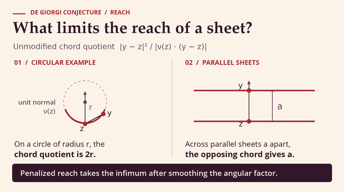
Normal lines from nearby points can intersect when a sheet bends. A second sheet can also enter the normal tube. The penalized reach measures both. For a regular zero with unit normal and another zero , the unmodified chord quotient is . It equals twice the radius of the normal-centered sphere through both points when the denominator is nonzero. For parallel sheets separated by a distance , a directly opposing point gives quotient . As a chord shrinks in a principal direction, the quotient tends to twice the reciprocal of the absolute principal curvature, if that curvature is nonzero.
The proof smooths the angular factor near a normal chord and takes the infimum over other zeros. A bounded-density window near the reach scale makes local regularity available even if global density is unbounded. The ensuing reach inequality and stability estimates control the weighted fourth curvature moment, squared defect and squared interaction, along with a count of poorly controlled zeros. For the six-dimensional sheets the bound has scale , where measures the largest energy density across centers at radius . The corresponding weighted area has upper scale . Keeping the same factor in both bounds lets the last argument discard rough regions at a controlled cost even as that factor grows.
9. The Radial Stability Argument That Rules Out Unbounded Density
Assume the normalized density is unbounded and let . At a center with energy comparable to the supremum, a ball of radius carries energy on the scale . The proof uses a common radial amplitude in the reach inequality and in an ambient stability test. It extends the amplitude normally from regular sheets and interpolates between adjacent sheets. The interpolation cost depends on the squared difference of their amplitudes. At the nearest gap, those amplitudes become nearly equal on the assigned side, leaving at most one side with an appreciable loss.
The ambient test retains more of the weighted defect than the preliminary surface test. Comparing the two inequalities gives a strict coefficient margin and forces a positive weighted integral to be small. Yet a fixed fraction of the energy in the selected ball can be assigned to regular sheet area. The long-reach part has too little area to account for it because disjoint normal tubes of substantial width would occupy too much volume. The reach cutoff is on the scale , which grows but takes up a vanishing fraction of . The remaining shorter-reach area gives a lower bound on that same integral, contradicting the upper bound. Finite density follows, completing the seven-dimensional classification.
10. From Allen–Cahn Energy to an Exact Minimizing Perimeter
Return to the eight-dimensional minimizer. The ball estimate in Section 6 ensures that the rescaled energies stay bounded locally. For scales tending to infinity, write and . The transition shrinks in the new coordinates. The rescaled energy balances against . Along a subsequence the fields converge locally in integral mean to a two-phase function equal to on a set and outside it.
The phase-transition lower bound gives at least the perimeter times the surface tension. To get equality, the paper patches a recovery sequence, which approximates a candidate phase with asymptotically optimal transition energy, to the original solution across a thin annulus. The proof splits the annulus into many layers and chooses one where the patch costs vanishing energy. Minimization and the resulting upper bound identify the whole limiting measure as , where is perimeter measure. Comparing with competing phase sets shows that locally minimizes perimeter. Energy monotonicity makes its limiting area ratio constant across radii, so the boundary is a cone. Exact convergence matters because an interface with flat support could otherwise carry extra energy.
11. Why the Directed Minimizing Cone Must Be Flat in Eight Dimensions
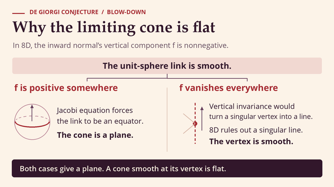
The increasing direction survives the blow-down. The inward normal has nonnegative vertical component on the regular part of the cone. An area-minimizing boundary in eight dimensions has singular set of dimension at most zero. A singular point away from the vertex would generate a whole ray under dilation, so the link , the intersection with the unit sphere, is smooth and compact. The translation Jacobi equation on the link is
Here is the Laplacian on the link and is its second fundamental form. If is positive on a component, integration forces its curvature to vanish. The component is an equator, and any further component would lie in an open hemisphere, which a closed minimal link component cannot do. If vanishes everywhere, the phase set is invariant under vertical translation. A singular vertex would then generate an entire singular line. Thus the cone is smooth at the vertex and equals its tangent hyperplane. In dimension nine the singular-set bound permits a line, precisely what appears in the cylindrical blow-down in Appendix A. Its interface is the product of the Simons cone in eight dimensions with the vertical line. The vertical normal component vanishes along its regular part. The connection between curvature and large-scale geometry also appears in Binary Verse AI’s coverage of spectral scalar curvature and Urysohn width.
12. How Unit Density Produces the Exact One-Dimensional Solution
A single plane carries normalized density one because its area in a ball is exactly the denominator’s geometric factor. The exact perimeter limit gives . Wang’s near-unit-density theorem then makes the original field one-dimensional. Write it as , with the orientation chosen so that and . The ODE conserves . The two distinct limiting values are stationary roots with equal potential, so they are and . Taking the positive square root and integrating recovers the translated hyperbolic tangent.
The scope is the stationary scalar quartic equation on all of Euclidean space. Other potentials and boundary-value settings pose separate classification questions.
The De Giorgi conjecture reaches its sharp monotone dimension here because the proof gets two separate facts to work together. Stable end profiles make the energy comparison possible, and directional information forces the resulting minimizing cone to be flat. Follow Binary Verse AI’s research explainers for more examples of what makes a PDE solution rigid, from interior regularity for the infinity Laplacian to critical points in the hot spots conjecture. For more PDE research coverage, see the Calderón inverse problem, forced Navier–Stokes and universal computation and global regularity for Vlasov–Maxwell.
What does De Giorgi’s conjecture say about the Allen–Cahn equation?
It asks whether a bounded entire solution of the stationary Allen–Cahn equation with an everywhere positive derivative in one fixed direction must depend on a single linear coordinate. The September 2026 preprint proves this in dimension eight for the scalar cubic equation under its stated hypotheses.
Wasn’t De Giorgi’s conjecture already proved in eight dimensions?
Savin proved the result through dimension eight under the additional assumption that the solution approaches the two constant wells at the opposite ends of the monotone direction. The new proof derives those limits from its other hypotheses.
Why does the eight-dimensional proof depend on stable solutions in seven dimensions?
The limits along the monotone coordinate are stable solutions in the seven transverse variables. The paper classifies those limits as constant wells or planar transitions. Both kinds of limits minimize energy and can be used as barriers to prove that the original eight-dimensional solution also minimizes energy.
How does the proof remove the energy-growth assumption?
It first proves rigidity for stable solutions with finite normalized energy density. In dimension seven, penalized reach, curvature estimates and a radial stability comparison then rule out unbounded density.
Why is dimension eight the critical threshold?
Nonflat minimizing cones exist in eight dimensions, but the cone produced by a monotone solution has a normal component of fixed sign in the monotone direction. That directionality and the dimension-eight singular-set bound force the cone to be a plane. In dimension nine the bound permits a singular line.
How does the proof obtain the hyperbolic-tangent solution?
Unit normalized energy density lets the proof apply Wang’s near-unit-density theorem and reduce the field to one variable. The increasing solution of the resulting ordinary differential equation is the hyperbolic tangent of the signed distance from the zero plane divided by the square root of two.
Does the proof also establish De Giorgi’s conjecture in dimension nine?
The conjecture fails in dimension nine and higher, where nonplanar strictly monotone entire solutions exist. Appendix A explains how the dimension-nine construction produces a cylindrical blow-down with a singular axis, consistent with the eight-dimensional proof.