
A manifold can extend forever while its geometry remains uniformly narrow in two directions. The new connection between scalar curvature and Urysohn width makes that intuition precise under a spectral condition that even permits negative scalar curvature locally. OpenAI’s October 5 paper proves that every complete, connected, smooth, boundaryless manifold of dimension satisfying admits a continuous map to an at-most--dimensional simplicial complex with uniformly bounded entire fibers. Crucially, their diameters are measured in the original metric. The proof explains how to obtain this conclusion without controlling an auxiliary weight at infinity.
Table of Contents
1. What OpenAI’s Spectral Scalar Curvature Proof Establishes
Theorem 1.1 in the original spectral scalar curvature paper gives one finite constant for each dimension. It works simultaneously for all manifolds satisfying the normalized hypothesis, including compact and noncompact examples. No orientability, spin structure, or bounded-geometry assumption is imposed.
| Item | Exact Scope |
|---|---|
| Dimension | |
| Manifold | Connected, complete, smooth, without boundary |
| Hypothesis | , as a quadratic-form inequality |
| Map | Continuous , with |
| Uniform Bound | Every whole fiber has -diameter at most |
| Positive Normalization | A lower bound gives |
Here denotes the original Riemannian metric. The scaling law matters: stronger spectral positivity controls fibers at a smaller length scale. The theorem establishes existence, without identifying an optimal constant or providing an efficient algorithm for constructing the map.
The OpenAI mathematics release announcement describes a broader collection of results and formalizations. It does not, by itself, certify this particular proof in Lean. The supplied manuscript presents an analytic and geometric argument.
To check the normalization, replacing by divides its Laplacian and scalar curvature by , while multiplying distances by . A spectral lower bound of therefore becomes one, and converting the resulting distance estimate back explains the inverse-square-root factor. This is a geometric scaling argument, not experimental data.
2. What Does Urysohn Width Actually Measure?
Urysohn width measures how much geometric information a continuous map can discard while keeping each inverse image small. For a metric space , the definition takes an infimum over continuous maps to simplicial complexes of dimension at most :
A simplicial complex is built from vertices, edges, triangles, and higher-dimensional simplices. It carries its usual polyhedral topology. The target need not be a smooth manifold. A fiber contains every point assigned the same output, including disconnected components.
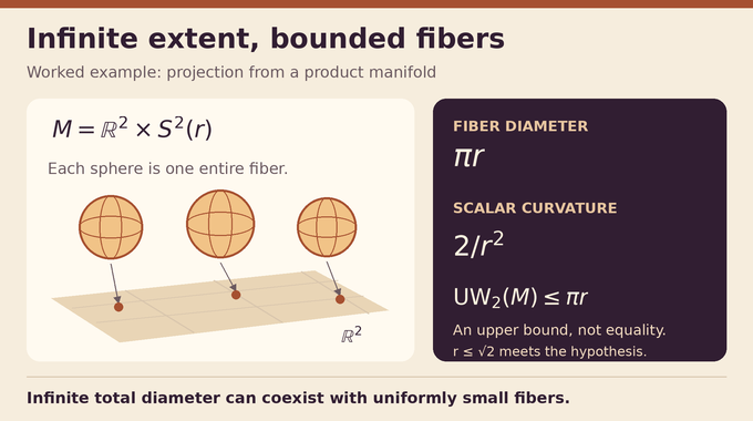
For a worked example, take the product , where is the round sphere of radius . Projection onto the plane has spherical fibers of diameter , although the product has infinite diameter. Its scalar curvature is , so ensures the normalized spectral condition. This gives an explicit upper bound on its Urysohn 2-width, not an equality or an optimality claim.
Bounding connected pieces separately would be weaker. Two tiny components assigned the same output could lie arbitrarily far apart. The theorem rules out that separation within every whole fiber.
3. Gromov’s Original Problem: Why Should Curvature Control Codimension Two?
The Gromov Urysohn width conjecture asks, in its relevant quantitative form, whether normalized positive scalar curvature forces uniformly bounded codimension-two width. Scalar curvature summarizes curvature through a scalar contraction of the Riemann curvature tensor. It gives much less directional information than sectional curvature, making such global control substantial.
The target dimension expresses a large-scale loss of two dimensions. It does not mean that the manifold changes its local dimension or becomes diffeomorphic to a lower-dimensional space. Nor does the theorem assert that its fibers are smooth two-dimensional surfaces.
The paper starts from the earlier positive scalar curvature and uniform codimension-two width theorem. It imports that work’s partition machinery and constructs new analytic inputs for it. Earlier results involving universal covers, topological restrictions, or bounds on connected level components have different scopes.
For readers approaching curvature through our Poincaré conjecture explainer, this is a useful distinction: the conclusion controls metric fibers rather than classifying topology. Our spacetime Penrose inequality analysis provides another setting where geometric hypotheses require careful separation from the final conclusion.
Uniformity is the demanding word. A finite width bound chosen separately for each metric would allow that bound to deteriorate across a family of examples. Here one constant must work across all permitted geometries in a fixed dimension, after the spectral normalization has fixed the unit of length.
4. Why the Spectral Curvature Condition Is More Difficult
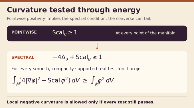
Use the sign convention . Multiplying the operator by a real smooth compactly supported test function and integrating by parts produces the defining quadratic-form inequality:
The quantifier is essential: this holds for every . Pointwise immediately implies it because the gradient term is nonnegative. The converse need not hold. Negative-curvature regions are permitted when the total quadratic form still satisfies the bound. Their size and placement cannot be arbitrary.
| Condition | What Must Be Controlled |
|---|---|
| Pointwise Positivity | at every point |
| Spectral Positivity | Curvature plus gradient energy for every compactly supported test function |
| Shared Conclusion | Uniformly bounded codimension-two Urysohn width for |
On a noncompact manifold, this definition does not assume that a lowest eigenvalue is attained. Treating the hypothesis as the existence of a global first eigenfunction would skip a necessary argument.
On a closed manifold, choosing the constant test function shows that average scalar curvature must be at least one. That necessary condition is not sufficient: the quadratic-form inequality must also survive every nonconstant test function. On a noncompact manifold, the constant function is generally unavailable because the tests require compact support.
5. From Spectral Positivity to a Positive Supersolution
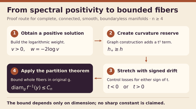
Lemma 3.1 supplies a smooth function satisfying . On a compact manifold, a positive first eigenfunction suffices. On a noncompact one, the proof uses Dirichlet first eigenfunctions on an exhaustion by relatively compact connected smooth domains.
Normalize those functions at one fixed point. The spectral hypothesis bounds their eigenvalues below by one, while a fixed test function bounds them above. Harnack inequalities and interior elliptic estimates give a subsequence converging smoothly on compact subsets to a positive limit. These estimates require no uniform geometry at infinity.
Set , and define the weighted scalar expression for a metric and smooth real function . Differentiating the logarithm cancels the gradient-square contributions:
The coefficient four is therefore structural. It converts operator positivity into exactly the weighted curvature expression used later. This use of elliptic estimates belongs to a broad analytic toolkit, also encountered in our Lane–Emden equation explainer, although the geometric objectives differ.
6. The Previous Obstacle: An Uncontrolled Logarithmic Drift
The positive supersolution solves the first problem but leaves the weight uncontrolled. Neither , its oscillation, nor its gradient has a global bound supplied by the hypothesis. Calling it a drift refers to the weighted divergence .
This matters because the proof must enlarge distances while preserving enough weighted curvature. A conformal change or direct reuse of earlier stretching estimates could introduce losses depending on precisely the quantities that are uncontrolled. Local regularity cannot be promoted into a uniform global estimate without justification.
The solution is to manufacture a reserve: a lower bound containing the square of a new drift. That positive term can absorb the losses of later metric changes. The proof never needs to establish a global bound for the old weight.
Readers of our local smoothing proof analysis will recognize the importance of tracking what an estimate actually controls. Here the decisive distinction is between compact-region estimates used for existence and constants that must depend only on dimension.
7. The First New Argument: Manufacturing a Quadratic Reserve
Proposition 3.2 starts with any complete metric and smooth . It solves a weighted prescribed-mean-curvature graph equation whose pressure is . The unknown height defines the enlarged graph metric .
Write and , the vertical angle factor. The density-preserving drift on the graph is . Subtracting the graph height gives .
The paper permits . Three square completions control terms involving level-set curvature, slope derivatives, and pressure. The remaining positive pressure-square and slope terms dominate , giving a constant independent of the original geometry and weight.
Existence is also addressed. Closed extensions supply approximate solutions, local height barriers confine them, and the graph-angle equation yields local gradient estimates. A diagonal limit produces the global graph. Completeness follows because the new smooth metric dominates the complete starting metric. The construction therefore creates the reserve without assuming bounded geometry at infinity.
There are two distinct uses of estimates here. Bounds depending on a fixed compact region allow the graph equation to be solved there. The final square-completion calculation removes that dependence from the reserve constant. Confusing those roles would incorrectly suggest an extra global hypothesis on the manifold.
8. The Signed Pressure Law That Makes Stretching Possible
The new drift can be negative as well as positive. Proposition 4.1 therefore constructs a pressure for every real drift value , with representing a height discrepancy. Its reserve is , with .
The pressure increases with discrepancy and diverges at two fixed endpoints, confining graph heights. Yet the simple choice fails: for positive , near a pole its discrepancy derivative becomes too large while . The curvature estimate needs a different sign there.
The proof instead prescribes discrepancy as an inverse function of positive pressure , then inverts. At small pressure it retains tangent-like behavior. At large pressure it changes the drift dependence, obtaining favorable control of . Odd extension in discrepancy treats negative pressure, while the estimates hold for both signs of drift.
This is not a cosmetic refinement. Moving a negative drift toward zero decreases its square. The later argument must remain valid through that decrease instead of assuming an ever-growing reserve.
9. Local Metric Stretching Without Losing Curvature Control
Lemma 5.1 enlarges the distance between a compact nonempty set and a closed nonempty set . A complete background metric fixes their initial separation and the support of the change. The current metric dominates .
The output satisfies and , with changes compactly supported in a prescribed neighborhood of . It raises separation to at least in the lemma’s working units. This number is an iteration factor, not the final width constant.
Curvature accounting retains , where . The losses consist of a small multiple of the metric-trace decrease, multiplied by , plus an arbitrarily small error of the same reserve scale. The trace decreases as the current metric grows.
At appreciable slope the graph enlarges lengths. Near zero slope, modifying the graph metric makes the curvature error small enough to absorb. Spatial cutoffs localize the deformation. These details allow many local operations without accumulating an uncontrolled curvature deficit.
The trace is taken relative to the fixed background during a round, starts at the dimension, and remains positive. Consequently its total decrease is bounded even if many operations affect one point. Resetting the background between rounds requires a separate rescaling argument, which is why a single local stretching estimate does not finish the proof.
10. How Repeated Stretching Produces Uniform Control
Choose maximal -separated centers in the original metric. Their closed radius- balls cover the manifold, and the radius- balls form a locally finite family. Completeness makes closed bounded sets compact, so a compact region meets only finitely many outer balls.
Each inner ball is paired with the complement of its outer ball. During one round, the background metric stays fixed. Trace decreases telescope, and adjustable errors have a summable total. This avoids requiring a uniform bound on how many neighborhoods overlap.
The positive-part term is crucial to the induction. If , then even for negative . Thus the reserve estimate survives when an increasing drift has a decreasing square.
Successive rounds use scales , restoring the reserve through rescaling. Every pair has its own finite target separation, so each label becomes inactive after finitely many rounds. Since all its changes stay inside one fixed outer ball, every compact neighborhood eventually stops changing. The resulting metric and drift are smooth, rather than merely weak limits, and satisfy .
If an outer ball already contains the whole manifold, there is a simpler case: the original diameter is at most , and a constant map works immediately. Otherwise all exterior sets are nonempty, so the separation construction applies. This case distinction prevents the iteration from being asked to separate a ball from an empty set.
11. From Stabilized Scalar Curvature to Bounded Urysohn Fibers
To reach the imported partition theorem, write as a locally finite sum of compactly supported functions. Divide each summand into sufficiently many equal log warps . Their sum stays , while their total squared-gradient cost becomes at most .
For the associated local circle products, the multiple-warp formula then gives:
Local finiteness means each neighborhood involves only finitely many nonconstant circle factors. No global infinite-dimensional product is required. Together with the prescribed separations, this supplies Theorem 2.1 with its precise hypotheses.
The partition construction assigns locally finite coordinates. Two points with the same output share a coordinate that confines their nearby reconstructed points to the same original outer ball. This bounds the whole fiber in , yielding . The dependence is only on dimension, without a claim of sharpness.
The related weighted cube inequality paper by Yuchen Bi develops another consequence of this research family. It is a separate result, not the source of Theorem 1.1. Likewise, the three-dimensional spectral Urysohn-width manuscript must be distinguished from this paper’s higher-dimensional proof.
The result connects scalar curvature and Urysohn width through a controlled sequence: spectral positivity supplies a weight, new graph constructions make stretching affordable, and an existing partition theorem delivers bounded fibers. For more proof-focused explanations, explore Binary Verse AI’s mathematics coverage and subscribe to our channel as we build an accessible research reference library.
What is the relationship between scalar curvature and Urysohn width?
Positive scalar curvature imposes constraints on the geometry of a manifold. The paper proves that the weaker spectral condition still guarantees uniformly bounded -dimensional Urysohn width for complete, connected, smooth manifolds without boundary of dimension at least four. Fiber diameters are measured in the original metric.
What is Gromov’s Urysohn width conjecture?
Its relevant quantitative form asks whether a uniform positive scalar-curvature lower bound forces a dimension-dependent upper bound on codimension-two Urysohn width. This paper extends the earlier pointwise result to a spectral curvature hypothesis.
Can scalar curvature be negative while the spectral lower bound remains positive?
Yes. A spectral lower bound is an integrated inequality involving curvature and the gradient energy of every compactly supported test function. It does not require scalar curvature to be positive at every point, although negative regions must remain compatible with the inequality.
Why does the proof use the operator ?
The coefficient four allows a positive supersolution to be transformed using . This produces the weighted scalar-curvature expression needed for the graph and metric-stretching arguments.
Why does OpenAI’s proof require a new signed pressure construction?
The logarithmic drift obtained from the spectral condition may be unbounded and have either sign. The signed pressure law permits controlled metric enlargement while managing curvature losses, including cases where increasing the drift decreases its square.
Does OpenAI’s spectral Urysohn width theorem apply in dimension three?
The supplied 27-page paper proves Theorem 1.1 for . A separate manuscript on dimension three establishes a spectral Urysohn 1-width theorem there. The two proofs and their dimension ranges should remain distinct.