
A black hole cannot be arbitrarily large while the universe around it carries arbitrarily little mass. Turning that intuition into a theorem has occupied relativists since 1973. OpenAI’s September 27, 2026 manuscript presents a proof of the spacetime Penrose inequality for a broad, precisely defined class of initial data, including moving configurations and disconnected trapped boundaries.
The crucial qualification is the area being measured: the least area of a full enclosure, rather than automatically the apparent horizon’s own area. The OpenAI spacetime Penrose inequality paper claims the sharp bound in every spatial dimension from three upward, with weaker decay requirements in three and four. It is a substantial preprint claim, not evidence that cosmic censorship itself has been proved or that this main theorem has been checked in Lean.
Table of Contents
1. The 1973 Penrose Conjecture: How Much Mass Must Surround a Black Hole?
Penrose’s argument connected gravitational collapse, the expectation that singularities remain hidden, and the principle that black hole horizon area does not decrease. If radiation carries energy away while a horizon persists, the initial configuration should contain enough mass to account for its eventual black hole.
That physical reasoning does not supply a rigorous theorem about an arbitrary spatial snapshot. Initial data consist of a spatial metric, describing distances, and extrinsic curvature, describing how the slice sits in spacetime. A proof must work with those quantities without assuming that the entire future evolution behaves conveniently.
An asymptotically flat end is a distant region where the geometry approaches Euclidean space at specified rates. It provides the reference structure needed to define total energy and momentum. The theorem concerns an exterior with a trapped inner boundary, rather than a complete history of gravitational collapse.
1.1. Spacetime Penrose Inequality: Key Facts
| Feature | Verified Manuscript Scope |
|---|---|
| Source | OpenAI manuscript dated September 27, 2026; Theorems 1.3 and 1.5. |
| Geometric Setting | Smooth, connected, orientable exterior, complete with its compact boundary included, and exactly one asymptotically flat end. |
| Mass and Area | Invariant ADM mass and the infimum of full enclosing-cut areas in the original metric. |
| Dimensions | All spatial dimensions from three upward under strong differentiated decay; weaker decay in three and four. |
| Verification Status | Released analytical proof claim. Related Lean artifacts do not formalize this main inequality. |
The 53-year interval describes the problem’s history, not how long an AI spent solving it. OpenAI’s October 6 release announcement identifies an internal frontier model as the source of the mathematical collection. It does not provide a paper-specific performance benchmark here.
2. What OpenAI’s Spacetime Penrose Inequality Proof Actually Establishes
In The Spacetime Penrose Inequality and Enclosing Area, write for ADM energy and for ADM linear momentum. These are asymptotic gravitational charges measured at spatial infinity. The invariant mass removes the contribution associated with overall motion:
Here is spatial dimension, is the area of the unit sphere of dimension , and is enclosing area. In three spatial dimensions, using geometrized units, the expression becomes:
The scaling is informative: quadrupling enclosing area doubles the minimum permitted mass in three dimensions. This is a lower bound, not a unique mass prediction. Larger masses remain compatible with the inequality. The units absorb Newton’s constant and the speed of light into the geometric quantities.
The dominant energy condition is , where and are the constraint energy and momentum densities. Both densities must be integrable. Weak future trapping means , with the normal pointing toward infinity. No sign is required of the other null expansion.
Theorem 1.3 assumes , , and , plus finite ADM limits, positive enclosing area and . The subscript counts controlled coordinate derivatives. Corollary 1.4 then removes the timelikeness assumption by deriving it.
Theorem 1.5, restricted to , needs only two metric derivatives, one tensor derivative and . Enclosing-area positivity and future timelikeness are conclusions there. The data remain smooth. These are weaker asymptotic requirements, not permission for arbitrary rough geometry. As with other major AI proof claims, the exact theorem controls the headline.
3. Why Earlier Penrose Inequality Proofs Could Not Handle General Spacetime
The Riemannian vs spacetime Penrose inequality distinction begins with , the time-symmetric case. The energy condition then gives nonnegative scalar curvature, and a marginal boundary becomes minimal. Those signs unlock powerful geometric flows.
Huisken and Ilmanen’s weak inverse mean curvature flow established a sharp three-dimensional bound for each connected component of an outermost minimal boundary. Bray’s conformal flow handled the total area of potentially disconnected horizons. Bray and Lee extended the numerical result through spatial dimension seven.
Geometric evolution also appears in the Hamilton–Perelman proof of the Poincaré conjecture, although Ricci flow is a different tool solving a different problem. Here the essential bookkeeping concerns mass and area.
When extrinsic curvature is nonzero, the useful scalar-curvature and boundary signs disappear. Jang-type graph deformations seek to recover them. Bray–Khuri’s generalized approach isolates favorable terms but leaves a divergence requiring simultaneous control. Jaracz’s nonexistence result rules out suitable smooth radial solutions for one zero-divergence coupling on particular spherical data. It does not rule out every generalized Jang strategy.
The history also includes sharp spacetime results under symmetry and other structural restrictions. A nonsymmetric three-dimensional result by Allen, Bryden, Kazaras and Khuri obtained an invariant-mass bound with a suboptimal constant under its assumptions. The new manuscript’s claimed advance combines the sharp coefficient with arbitrary extrinsic curvature in its stated class.
4. The Hidden Problem With Black Hole Horizon Area
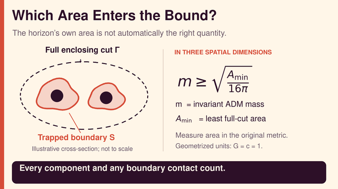
A surrounding surface can have less area than the apparent horizon it encloses. Curved geometry is not obliged to honor the intuition developed by wrapping boxes. Ben-Dov constructed examples satisfying the dominant energy condition where a direct apparent-horizon-area bound fails. Carrasco and Mars found a separate obstruction involving generalized apparent horizons, even with an outer area-minimizing generalized horizon.
The enclosing area Penrose inequality therefore specifies its admissible surfaces carefully. A full enclosing cut is the entire compact, smooth, embedded, two-sided intrinsic boundary of a connected, closed outer domain containing the sufficiently distant end. Every component counts. Portions coinciding with the original boundary also count.
The infimum of their areas, measured using the original metric, defines . The original boundary itself is admissible. A competing cut need not be connected, trapped or minimal, and the infimum need not be attained. Dropping a component or boundary-contact patch would change the mathematical question.
This distinction also limits the physical shorthand. A trapped boundary is supplied by the initial data. An event horizon is defined using the spacetime’s global causal structure. The theorem does not reconstruct that event horizon or identify every admissible enclosing cut with a physical black hole surface.
5. Step One: Preparing the Spacetime Geometry Without Losing Mass or Area
The argument first replaces the distant end with a vacuum reference end whose ADM charges match the original data. It then bends that reference slice toward a rest configuration and repairs errors in the Einstein constraint equations. Simply declaring momentum zero would change the problem. The construction has to justify the mass comparison geometrically.
The prepared output has compactly supported extrinsic curvature, a strict dominant-energy margin and strictly negative future boundary expansion. Strictness provides room for later perturbations. Vacuum describes the reference model, not an assumption that the original exterior contains no matter.
Area control must hold for every full enclosing cut, including surfaces reaching into the modified end. Comparing only the original horizon would leave a gap. The weaker-decay preparations in three and four dimensions require different transfer arguments. The common deformation theorem is applied at finite preparation stages, then numerical comparisons return the conclusion to the original data.
In the three-dimensional preparation, the enclosing infima converge to the original one. In four dimensions, the proof establishes the lower comparison it needs. It does not claim that every intermediate enclosing-area definition becomes identical. Keeping the direction of comparison is enough for the bound.
6. Step Two: The New Graph–Conformal Identity That Controls Curvature, Mass and Area
The main deformation uses a graph height , a conformal variable , and a positive warping function :
The graph contribution adds a nonnegative quadratic form to the metric. Keeping therefore prevents lengths, and consequently enclosing areas, from shrinking too much. Independently, the curvature identity organizes the energy condition, controlled quadratic terms and a divergence:
Here is a normalized graph gradient with length below one, is a modified trace, , and is a positive weight. The vector field carries the divergence flux. The controlled quadratic expression bounds relevant derivatives through weighted coercivity estimates.
The energy condition makes nonnegative. A modified trace equation and a deliberately nonzero divergence source then coordinate curvature, the conformal floor and mass change. The breakthrough being claimed is their compatibility. A favorable algebraic identity alone would not establish solvability.
The modified conformal variable packages height distortion into the scalar unknown:
This change of variables is part of the design of the equations. It links the conformal factor to graph slope instead of treating the two deformations as independent corrections. Their interaction is exactly where protecting area while controlling mass becomes difficult.
7. Step Three: Solving the Coupled Nonlinear Equations
The paper solves for height and a modified conformal unknown . Its coupled system includes:
The source allocates a small share of the coercive quadratic and height-gradient terms, spends part of the strict energy margin, and includes a negative penalty near the forbidden conformal floor. That penalty helps curvature but can increase mass. Its integrated contribution must become negligible.
Height barriers and the floor argument supply lower control. Testing the divergence equation and using a graph Sobolev inequality produces a polynomial upper bound before uniform ellipticity is available. These estimates control graph distortion. Separate gradient and regularity arguments then address the trace equation’s gradient-aligned coefficients and the divergence equation’s quadratic gradient growth.
Fixed-point continuation uses two homotopies on large truncations, with zero outer data. Exhaustion extends solutions to the filled manifold. This is an existence proof, not a demonstrated numerical solver or a black hole simulation benchmark.
The order of estimates matters. Assuming uniform ellipticity to obtain the very bounds needed to establish it would be circular. Likewise, a constant allowed to grow arbitrarily with the large parameter cannot replace a polynomially controlled constant in the final mass estimate. The manuscript distinguishes these two kinds of control.
The scales and make both and equal . At fixed positive , exponential decay beats the polynomial losses in . Uniform control, also central to the logic of spectral-gap lower bounds, is what makes a limiting argument useful.
8. Step Four: Constructing a Minimum-Area Enclosure Outside the Filled Region
Filling the inner boundary eliminates an unwanted inner flux in the divergence equation. It creates a new danger: an area-minimizing enclosure could wander into the artificial filling, where the energy condition was never imposed. Such a surface would not justify the intended comparison.
The proof separates the filling by height, then applies an additional conformal change that inflates area deep inside while remaining controlled toward infinity. Perimeter minimization selects an enclosure. Density estimates and detachment from a distance obstacle locate its frontier in the region with suitable scalar curvature.
8.1. Three Estimates the Construction Must Preserve
| Quantity | Required Comparison |
|---|---|
| Scalar Curvature | Nonnegative outside the selected minimizing frontier, with the required integrability and decay. |
| ADM Energy | At most the prepared energy plus a polynomial times exponentially vanishing errors. |
| Full Frontier Area | At least , counting every component, where is prepared enclosing area. |
All three estimates are necessary. A curvature improvement that sacrifices area, or an enclosure that enters the uncontrolled filling, would not recover the sharp inequality.
Perimeter is the appropriate weak notion of area when minimizers may have singularities. Local minimization constrains small changes on either side of the frontier. Outer minimization controls larger enclosing competitors. These properties serve different roles and must both survive the construction.
9. Step Five: Recovering the Sharp Penrose Mass–Area Bound
The constructed exterior now meets a Riemannian comparison theorem. Through dimension seven its minimizing frontier is smooth. In higher dimensions it can have a singular set of Hausdorff dimension at most . The required treatment comes from the companion minimizing-frontier argument, rather than an unqualified reuse of a smooth-boundary theorem.
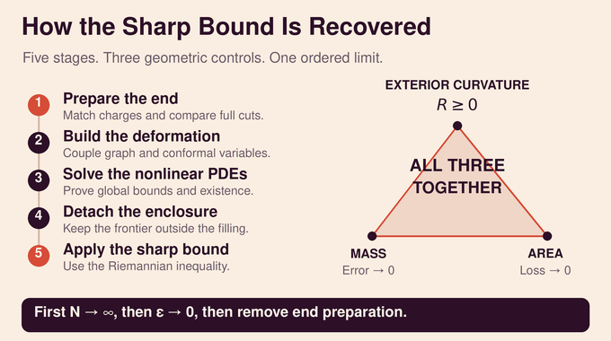
For prepared energy and enclosing area , first send to infinity at fixed positive . The error in energy disappears, giving:
Next let decrease to zero, then remove end preparation. The sharp coefficient survives because both area loss and mass error vanish in the controlled order. No metric at infinite is required. As in other sharp geometric inequalities, identifying the exact constant is a stronger achievement than obtaining some positive bound.
Reversing these limits would require estimates the argument has not supplied. At each fixed preparation stage and positive tolerance, the smooth construction produces a numerical inequality. Passing those inequalities onward avoids asserting convergence of the entire geometric construction.
10. What the Proof Resolves and What It Does Not
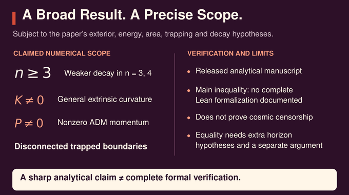
The claimed numerical theorem permits arbitrary extrinsic curvature, nonzero ADM momentum and disconnected weakly future trapped boundaries. It imposes no spin, vacuum or interior-topology restriction within its stated exterior class. Schwarzschild–Tangherlini exteriors attain equality, demonstrating sharpness.
Classifying every equality case is harder. The separate equality-and-rigidity manuscript imposes additional horizon hypotheses and varies the original data to recover a Schwarzschild–Tangherlini slice. Equality in an auxiliary comparison metric does not automatically identify the original spacetime geometry.
For AI readers, verification remains specific to the result. The repository’s formalization notes cover related Bondi-end replacement and Schwarzschild examples. They explicitly retain a conditional use of the asymptotically flat inequality, rather than proving this main theorem. Proof discovery and Lean formalization are distinct achievements.
A useful audit follows dependencies: check the precise theorem, the estimates supplying existence, the area comparison and the endpoint theorem. A repository link or a successful formal check of a neighboring result cannot replace those steps.
The practical contribution is a proposed analytical bridge from general initial data to sharp Riemannian geometry. It supplies no measured improvement in simulations or observations and does not establish cosmic censorship. Researchers assessing the spacetime Penrose inequality should inspect the coupled-equation estimates, enclosure transfer and companion endpoint together. Follow Binary Verse AI’s coverage of AI mathematical proofs for source-led explanations that keep theorem scope and verification visible.
11. Frequently Asked Questions About the Spacetime Penrose Inequality
What is the spacetime Penrose inequality?
It relates the invariant ADM mass of asymptotically flat initial data to an enclosing area associated with trapped regions. In three spatial dimensions, the paper proves under its stated hypotheses.
Has OpenAI solved the Penrose conjecture?
The September 2026 paper presents a proof of the sharp enclosing-area formulation for specified smooth, asymptotically flat initial-data exteriors. It extends beyond time-symmetric geometry. This is a published preprint claim requiring independent scrutiny, and it does not establish every possible formulation of the Penrose conjecture.
Why was the spacetime Penrose inequality so difficult to prove?
Earlier general Riemannian proofs used time symmetry, where extrinsic curvature vanishes. For general spacetime data, a deformation must simultaneously control scalar curvature, preserve a useful mass comparison and protect enclosing area. Coordinating those requirements was the central obstruction.
Why does the proof use enclosing area instead of apparent horizon area?
Known counterexamples invalidate certain inequalities using apparent-horizon area or generalized-horizon area directly. The paper instead takes the infimum over admissible full enclosing cuts, counting every component and all portions coinciding with the original boundary.
What is the key mathematical breakthrough in OpenAI’s proof?
The paper constructs a coupled graph–conformal deformation with a controlled nonzero divergence source. Together with global estimates and a minimizing-enclosure argument, it converts the stated spacetime initial data into geometry suitable for applying a sharp Riemannian inequality.
Does the Penrose inequality proof establish cosmic censorship?
No. Cosmic censorship motivated Penrose’s mass–area argument, but proving this inequality is not equivalent to proving cosmic censorship. The theorem establishes a geometric mass bound for initial data satisfying specified assumptions, not the global fate of every gravitational collapse.
Has OpenAI’s spacetime Penrose inequality proof been formally verified in Lean?
The checked repository notes do not document a complete Lean formalization of this paper’s main inequality. The related formalization notes describe Bondi-end replacement and Schwarzschild equality examples. A supporting result assumes the asymptotically flat exterior Penrose inequality, and the general Bondi–Penrose inequality also remains unformalized.