
Imagine controlling a small accessible patch of an object while its remaining boundary stays out of reach. Can those measurements determine its entire hidden geometry, together with a rule for transporting two-component complex vectors? OpenAI’s October 5, 2026 manuscript answers this version of the Calderon Inverse Problem with a uniqueness theorem. For a smooth metric and smooth unitary connection in dimension at least three, identical responses on that patch force equivalence by coordinate and frame changes fixed there. This is an exact mathematical identification result, not a demonstrated imaging system. Its central difficulty is making a matrix-valued continuation argument survive as probing spheres shrink.
Table of Contents
1. What Is the Calderon Inverse Problem, and Why Does One Boundary Patch Matter?
Calderón’s original inverse boundary value problem asks whether electrical boundary measurements determine an interior conductivity. In the anisotropic Calderon problem, direction-dependent material behavior corresponds to geometric information. Here, the unknown geometry is a Riemannian metric, which assigns lengths and angles inside a manifold.
Full boundary data allow excitation and observation everywhere. A partial data Calderon problem restricts access. This paper places both on the same nonempty open patch, denoted . Think of varying signals through one accessible window and recording responses there, with zero prescribed input elsewhere. The theorem uses every smooth patch-supported input, not a finite sensor experiment. Boundary conditions also drive the distinct question explored in our Hot Spots Conjecture explainer.
| Feature | Verified Scope |
|---|---|
| Primary source | Determination of a metric and a unitary connection from one boundary patch, October 5, 2026 |
| Domain | Compact connected smooth manifold with nonempty smooth boundary, dimension |
| Unknowns | Smooth metric and arbitrary smooth unitary connection on the trivial Hermitian rank-two bundle |
| Data | Zero-frequency energy form on the same nonempty relatively open proper boundary patch |
| Conclusion | Uniqueness up to a diffeomorphism and unitary gauge fixed on that patch |
| Practical scope | No numerical reconstruction or noise-stability theorem supplied |
2. What OpenAI’s One-Patch Proof Actually Establishes
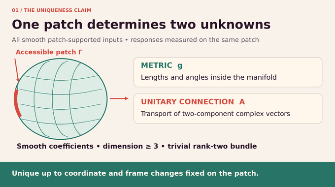
Theorem 1.1 compares two coefficient pairs on the same manifold. If their measured energy forms agree for every pair of smooth, compactly supported patch inputs, a smooth diffeomorphism and smooth unitary matrix field satisfy:
The star on denotes pullback. The matrix is the two-by-two identity. A diffeomorphism changes coordinates. A unitary gauge changes the orthonormal frame in each complex fiber. Both preserve the observations when fixed on the patch. As a worked invariance example, choose any smooth interior frame rotation equal to identity near the boundary. Applying the displayed connection transformation produces identical data despite changing its matrix coefficients. The theorem says these inherent ambiguities exhaust the possibilities.
For a concrete example, take the Euclidean unit ball with zero connection. Choose a real smooth function supported strictly inside it and set . Then is generally nonzero. Nevertheless, carries each original harmonic solution to its transformed solution, and unitarity preserves the energy pairing. Boundary measurements cannot distinguish these two coefficient descriptions. This illustrates gauge ambiguity without invoking noise or limited experimental precision.
3. The Measurement Equation: Connection Laplacians and the Dirichlet-to-Neumann Map
Write , where is a one-form taking values in skew-Hermitian two-by-two matrices. The connection Laplacian and its Dirichlet problem are:
The adjoint uses the metric and Hermitian fiber product. Zero frequency means there is no varying spectral parameter. The zero-Dirichlet operator is invertible: a zero-energy section is parallel, and zero boundary trace makes it vanish. The local Dirichlet to Neumann map is encoded by:
Here is metric volume density, and means smooth functions with compact support. The product is linear in its first argument. This energy formulation avoids assuming the unknown boundary metric or its surface measure is already available. Densities also remove any orientability requirement.
4. Why Previous Calderón Results Could Not Establish This Joint Recovery
The manuscript places its result beyond several earlier settings. Sylvester and Uhlmann’s classical uniqueness theorem treats smooth isotropic conductivity in dimension at least three. Earlier anisotropic and joint geometric recovery results used real analyticity or other restrictions. Analytic coefficients are much more constrained than arbitrary smooth coefficients.
Connection recovery also had important results with a known metric, special geometry, or a Yang–Mills condition. The present unitary connection inverse problem leaves the smooth metric unknown and imposes no Yang–Mills equation. It adapts continuation machinery from a scalar companion manuscript, but does not apply scalar uniqueness directly to matrix boundary data. Regularity assumptions matter here, just as they do in the different setting of infinity-Laplacian regularity.
5. Step 1: Recovering Boundary Jets Through Symbol Factorization
First choose boundary-normal coordinates and a gauge with zero normal connection component. Factorizing the differential operator yields the complete local symbol of the boundary response. For tangential metric matrix and tangential covector , the leading density-valued symbol is . Its square determines .
Because the tangential dimension is at least two, the determinant recovers from . Lower symbol terms separate by parity: metric contributions are even under , while the new connection contributions are odd. Recursive comparison determines every normal derivative and hence every boundary Taylor jet. Crucially, matching all jets of smooth coefficients does not imply equality in an interior collar. The next construction supplies a different starting region.
6. Step 2: From Local Boundary Measurements to Matching Green Matrices
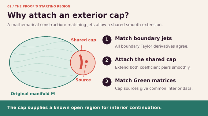
Attach a small exterior cap through a smaller patch inside . The matching jets permit a shared smooth extension of both coefficient pairs into this cap. They need not agree immediately inside the original manifold.
For a source supported in the cap, the corresponding solution minimizes a coercive energy functional. Replacing its original-interior part by the other system’s harmonic extension preserves that energy because the boundary forms agree. Reversing the comparison proves equality of the cap solutions. Varying the sources yields equality of the Dirichlet Green matrices there, away from their diagonal. These matrix kernels describe the response at one point to a vector source at another. The cap converts inaccessible interior identification into a continuation problem with known interior starting data.
7. Step 3: How Harmonic Frames Identify Interior Points and Fibers
Evaluate all common cap-source solutions at an interior point. These evaluations distinguish different points, span every fiber value, and realize every two-jet compatible with the homogeneous equation. A two-jet consists of value, first derivatives, and second derivatives.
Invertible matrices made from harmonic columns supply local harmonic frames. They eliminate the zeroth-order term, although they need not be unitary. The evaluation identities define a unique maximal match: a local isometry together with a unitary fiber identification. Distinct candidate images would contradict independent control of values at two points. If this match stops, the proof prepares coordinates and harmonic frames near a frontier point. It must then show that the equations agree across that apparent stopping place.
8. Step 4: Continuing Green Matrices with Carleman Estimates
A mixed Green matrix satisfies separate elliptic equations in its two variables, with matrix actions on different fiber indices. Initially it is known on a cross-shaped product region. Lemma 3.1 extends such data if each variable admits an interpolation inequality:
The sets are larger domains, observed subregions, and target subregions. The exponents measure quantitative propagation of information. A singular-function expansion has terms bounded by powers , where the positive singular values decay faster than any fixed inverse power. The strictly positive exponent makes the extension series summable.
Carleman estimates provide the interpolation inequalities under a strict geometric Hessian condition. Summing scalar estimates over vector components permits absorption of bounded matrix lower-order terms. Gluing the resulting extensions requires controlled overlaps. This is a geometric use of quantitative PDE estimates, a different mechanism from the oscillatory estimates discussed in our local smoothing explainer.
The threshold is more than a technical decoration. Separate uniqueness alone says that an already existing solution is determined by open-set values. It does not automatically construct an extension outside its original domain. Here, the interpolation exponents and singular-value decay establish convergence of a candidate extension, while unique continuation identifies that extension with the original data on the required overlaps.
9. Step 5: Shrinking Geodesic Spheres and Matrix-Valued Harmonic Transfer
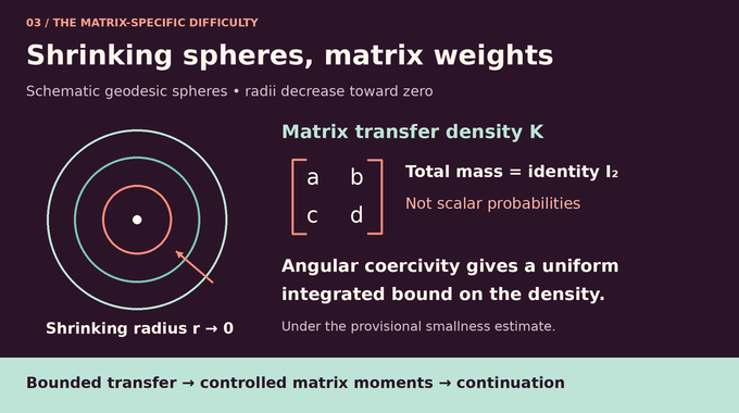
The continued kernel transfers first-system harmonic functions to second-system ones across moving geodesic spheres. The reference metric has inverse . The second inverse metric is rescaled to . Thus has zero -trace. This isolates conformal scale from the principal-tensor comparison.
Here is the tangent unit sphere, its probability measure, and the chosen radius. The density acts from the left. Its total mass reproduces constant columns. It is a matrix density, not a scalar probability distribution.
Existence at every positive radius does not ensure boundedness as radii shrink. Angular coercivity supplies the missing control. Applied to the sphere-mean-zero quantity , the system estimate absorbs matrix perturbations and yields a uniform integrated bound . The cutoff selects the relevant base region . This is conditional on derivatives of through order eight being bounded by a small multiple of the radius. The next step improves that provisional comparison.
The sphere geometry is chosen to preserve the strict Hessian condition during motion. A concave depth function determines the radius profiles, while known regions provide the initial and cutoff data. The order of choices matters: fixed geometric margins come first, and the final spatial dilation comes later. Otherwise constants could deteriorate as the spheres collapse, invalidating the improvement needed below.
10. Step 6: How Matrix Moments and Conformal Killing Theory Complete the Difficult Estimate
Scalar harmonic coordinates can remove first moments. Matrix-valued first moments survive a harmonic frame. Define displacement matrices , independent of the shrinking parameter, using the paired coordinate matrices :
Repeated spatial indices are summed. The selected harmonic columns span allowable jets, and is their remainder. Taylor expansion and the density bound control weighted square-integrable norms of and . Interpolation initially gives bounds for displacement derivatives and bounds for remainder derivatives, through order ten.
Comparing the harmonic equations, then testing trace-free Hessians with zero gradient, produces the exact projected system:
The projection is . The drifts are matrix coefficients of the normalized first-order terms. Their contribution retains multiplication order:
The error is through eight derivatives. Apply the real-linear matrix projection . Writing , with real , removes . Coordinate normalization determines algebraically from . The remaining first-order system has conformal Killing principal part, componentwise.
In these Euclidean identities, Z is the homogeneous cubic vector field used to test injectivity on third derivatives, and the Kronecker delta is the identity tensor. They explain finite type. Taking a trace forces , and dimension at least three then forces its Hessian to vanish. Two prolongations therefore determine third derivatives from lower jets. Starting from zero displacement on the known side, the resulting finite-dimensional differential system and Gronwall’s inequality improve displacement through nine derivatives. Substitution into the projected equation gives:
The extra half-power is decisive: relative to the assumed small positive multiple , the error ratio tends to zero. This closes the shrinking-sphere argument.
The projection deserves care: it removes real scalar matrices, rather than all complex scalar matrices. In particular, an imaginary multiple of remains among the components of . After this projection the equation is , where contains no derivatives. This precise decomposition lets the finite-type argument control the entire remaining matrix displacement, without silently discarding a connection component.
11. Step 7: Removing the Conformal Factor and Proving Global Uniqueness
Fix the geometry, thresholds, and radius profiles before choosing one sufficiently small spatial dilation. The improved estimate makes the provisional comparison strictly stronger. An open-and-closed argument extends it to every positive shrinking parameter. Letting radii collapse gives equality of normalized principal tensors and harmonic-frame drifts, leaving only conformal metric scale.
Write , set , and denote harmonic-frame connections by . Operator comparison yields:
Here the scalar Laplacian uses the divergence-of-gradient sign convention. On the known side, . Unique continuation makes it one throughout the connected neighborhood, so the metrics agree exactly. The intertwiner stays unitary by connection parallel transport.
Every proposed interior frontier can now be crossed, contradicting maximality. Compactness and source evaluations establish surjectivity. Metric completion and normal flow extend the isometry smoothly to the boundary. Finally, arbitrary patch-supported traces force both transformations to be identity on every component of . Riemannian metric recovery here concerns the whole metric, unlike the geometric quantities discussed in our scalar curvature and Urysohn width guide.
The continuity argument also avoids changing the problem while taking the limit. The displacement, selected harmonic columns, and coefficient differences remain fixed as the radius parameter varies. At each positive parameter the strict improvement persists nearby, while compactness supplies closedness. Consequently the same equations satisfy the estimates down to arbitrarily small radii, forcing exact equality rather than agreement only along a changing sequence of rescaled problems.
12. What the One-Patch Proof Does and Does Not Resolve
| Established in the Manuscript | Not Established Here |
|---|---|
| Exact smooth uniqueness modulo the stated symmetries | A stable reconstruction method from noisy finite data |
| Trivial Hermitian rank-two bundle, dimension at least three | The corresponding theorem for arbitrary bundle ranks or dimension two |
The Family 365 formalization scope note describes a different result: bounded-measurable scalar conductivity nonuniqueness in three dimensions. Its Lean source entry point culminates in a scalar nonuniqueness theorem. Neither supplies a Lean verification of this joint smooth recovery proof. As with our Navier–Stokes formalization coverage and Fermat formal proof explainer, formalization claims must track the actual statement encoded.
The Calderon Inverse Problem contribution is the mechanism linking local observations to global identification: bounded transfer, controlled matrix moments, finite-type improvement, and removal of conformal scale. Turning that uniqueness into reliable computation remains separate work. Follow Binary Verse AI for research explainers that connect theorem statements to the estimates that make them possible.
Can the Calderón inverse problem be solved using only one boundary patch?
For the smooth metric-and-connection setting of this paper, Theorem 1.1 establishes uniqueness from any nonempty relatively open proper boundary patch. Both inputs and observations remain on that patch. Recovery is up to a diffeomorphism and a unitary gauge that equal the identity there.
What does the Dirichlet-to-Neumann map measure in OpenAI’s proof?
It describes the boundary response to prescribed Dirichlet data for the connection Laplacian. The paper encodes that response as a sesquilinear energy form without presupposing a known boundary metric or boundary measure.
Why can the metric and unitary connection only be recovered up to gauge and diffeomorphism?
Coordinate changes and unitary changes of frame preserve the measurements when they equal the identity on the measured patch. The theorem proves uniqueness modulo these unavoidable transformations.
What is the hardest mathematical step in the one-patch uniqueness proof?
The manuscript identifies the matrix-valued first moment of harmonic transfer as its main matrix-specific difficulty. A harmonic frame does not normalize it away. A projected displacement equation with conformal Killing principal part and its finite-type property provide the stronger estimates needed for continuation.
Why does the theorem assume dimension at least three and a rank-two bundle?
The boundary-symbol recovery and conformal Killing argument use the dimension restriction. The theorem is stated and proved for the trivial Hermitian rank-two bundle. The manuscript does not establish the corresponding result for arbitrary ranks or two-dimensional manifolds.
Does OpenAI’s proof provide a practical reconstruction algorithm or a Lean-verified proof?
The manuscript provides neither a demonstrated numerical reconstruction algorithm nor a stability theorem. The linked Family 365 Lean formalization concerns a separate bounded-measurable scalar conductivity nonuniqueness result, rather than this joint metric-and-connection recovery theorem.