

Three tables can have identical row and column totals yet receive very different probabilities from a careless random generator. Contingency table sampling asks for something stricter: every feasible integer table must have the same chance. OpenAI’s September 24, 2026 manuscript establishes exact uniform sampling for arbitrary nonnegative margins, with polynomial expected bit complexity. Its route is surprising: build a bounded approximate sampler, calculate its remaining bias on an exceptionally rare branch, and cancel that bias exactly. The randomness consists of fair bits throughout. What begins imperfect is the intermediate output distribution, not the random source.
Table of Contents
1. What Is Contingency Table Sampling With Fixed Margins?
A contingency table is a matrix of nonnegative integers. Write for its row totals and for its column totals. Both sum to the same grand total . The feasible set is
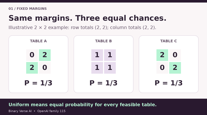
Uniform sampling of contingency tables assigns probability to every member. Fix both row totals and both column totals at two. Choosing the upper-left entry determines everything else: it can only be zero, one, or two.
| Feature | Guarantee |
|---|---|
| Input | Arbitrary nonnegative integer row and column margins with equal totals |
| Dimensions | Both row and column counts may vary |
| Approximate output | Total-variation error at most for requested integer |
| Approximate cost | Polynomial worst-case bit time in |
| Exact output | Equal probability for every feasible table, with almost-sure termination |
| Exact cost | Polynomial expected bit time in |
| Upper-Left Entry | Complete Table | Uniform Probability |
|---|---|---|
Each displayed matrix has row sums and column sums of two. Fisher’s exact test uses a different conditional distribution, so its probabilities need not match these equal weights. Specifying fixed margins alone does not specify a probability law.
In a larger table, choosing each locally feasible entry uniformly need not produce a uniform final matrix. One early choice may admit many more completions than another. A correct sampler must account for that imbalance. The small example is unusually simple because each permitted first entry has exactly one completion.
2. Why Earlier Algorithms Could Not Handle Arbitrary Margins
The manuscript’s introduction separates several successful but restricted approaches. Two-row algorithms already achieved polynomial approximate sampling, and monotone coupling from the past gave exact sampling with an expected bound stated using uniform real draws. Fixed-row methods extended approximate counting, rejection sampling, and heat-bath mixing, but their polynomial bounds depended on keeping the row count fixed.
Sparse exact generation required a genuine restriction involving the largest margin. Dense methods exploited transportation-polytope geometry when margins were large. Neither regime covered every combination of tiny and enormous margins with both dimensions varying. The paper’s solution combines these complementary strengths rather than assuming the entire input is dense.
A divide-and-conquer construction used few expected random bits, but its cited polynomial total-runtime conclusion depended on efficiently evaluating parity-restricted counting quantities. An arithmetic-operation bound also leaves open the cost of manipulating long integers. This distinction matters whenever counts become huge, as in counting perfect matchings. The new claim accounts for random bits and integer arithmetic together.
3. What Does OpenAI’s Exact Uniform Sampling Proof Establish?
Theorem 1.1 in the original sampling manuscript gives two algorithms. For any requested integer , the first always finishes within polynomial time and produces a feasible table whose distribution differs from uniform by at most in total variation. That distance is half the sum of absolute probability differences across all tables.
The second produces an exactly uniform table, terminates almost surely, and has polynomial expected bit cost. The polynomial is uniform over all margin vectors. Positivity, balance, sparsity, and fixed dimension are unnecessary. These are mathematical guarantees, not reported throughput measurements or a practical software benchmark.
Binary encoding is decisive. A margin of size needs 101 binary digits, while a loop proportional to that numerical value is enormous. The bound depends polynomially on instead. OpenAI’s mathematics release announcement supplies publication context. The manuscript supplies this theorem’s assumptions and proof.
4. Splitting Small Margins From the Large Rectangle
Section 2 introduces deliberately generous parameters:
Here controls dimension, is padding, is the small-margin threshold, and caps large completion coordinates. Rows and columns with original margins at least determine a complete rectangle . Every other cell belongs to the small-slot set . Its entry is bounded by an incident margin below .
Only small slots become explicit chain coordinates. Each stores a row viewpoint and column viewpoint , with doubled coordinates between zero and . Agreement means . Keeping both viewpoints permits carefully controlled temporary discrepancies.
The large rectangle is handled through conditional completions. It never becomes a collection of explicitly explored enormous entry ranges during an ordinary run. A fixed feasible starting table comes from greedily exhausting rows or columns. Empty blocks and singleton dimensions have deterministic conventions, preventing edge cases from becoming hidden assumptions.
This separation is about representation as much as geometry. The threshold is polynomial in dimension, so explicit small coordinates remain bounded independently of the numerical grand total. Large entries may require many possible values, but writing any one value still needs only its binary digits. The algorithm exploits that difference throughout.
5. How Padding and Completion Weights Preserve Uniformity
After fixing a small state, subtract its row and column contributions to obtain original residual margins. Add for each large cell incident to the corresponding row or column. Every nonempty completion margin is then at least , even when the original input mixes radically different scales.
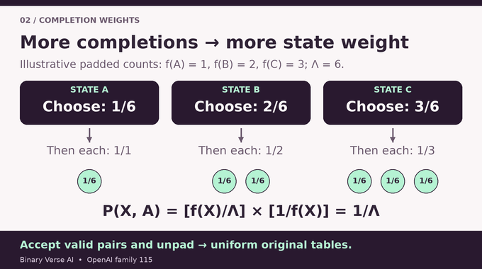
Let be the padded completion set for a feasible small state , and let . Across all feasible small states, define
Draw according to this stationary law, then draw a completion uniformly from . The cancellation is exact:
States with many completions appear more often, compensating for the smaller probability of each individual completion. This counting-to-sampling relationship also motivates counting common bases of two matroids. Here the bounded sampler never evaluates completion counts directly. It tests proposed moves by drawing completions instead. Successful pairs must also pass the unpadding test before becoming original tables.
6. Repairing Defect States Without Losing Valid Tables
A transversal has agreement at every small slot. A defect has one positive discrepancy, , and one negative discrepancy, . Their total discrepancy cancels, preserving equality between residual row and column totals. The enlarged graph includes local unit exchanges and designated repair edges.
For negative slot and positive slot , repair uses the corner . It removes one unit from the positive row viewpoint. If is small, it adds that unit there and balances the viewpoints. If is large, the completion receives the corresponding unit instead.
Lemma 2.1 proves feasibility and an injection for each ordered defect type. Therefore , where is the repair. If denotes total transversal weight, Proposition 2.3 gives
Success requires a transversal and every large completion entry at least . Subtracting padding then gives an original table. The paper bounds failed unpadding by comparing unrestricted enlarged tables, and proves that successful pairs correspond bijectively to original tables. Conditional uniformity survives rejection.
The injection is stronger than merely finding some feasible repair. If many defects could collapse onto one transversal without a multiplicity bound, defects might dominate the stationary mass. Fixing the ordered discrepancy locations makes repair injective, and counting those possible locations limits the total distortion. That bound makes repeated recovery attempts affordable.
7. The Quadratic Signature Argument Behind the Proof
The central algebraic task is to control neighboring conditional distributions. Section 3 first softens feasibility: configurations receive positive weights penalizing margin violations, with infeasible contributions vanishing as a parameter tends to zero. This permits comparisons before taking the hard-constraint limit.
The weight factors are log-concave sequences attached to a laminar family of coordinate sets. Laminar means that two sets are either disjoint or one contains the other. Separate row and column viewpoints create precisely this structure. The connection to log-concave sampling is geometric, but the required closure statement is proved specifically for these integer coordinates.
A two-removal matrix records weights after removing two coordinate units from a display with two excess units. Removing twice at the same coordinate produces a diagonal entry. These matrices have at most one positive eigenvalue. Balanced-pair summation preserves that signature through a discrete second-difference calculation with explicit endpoint treatment. Arbitrary sums do not preserve it. The proof also avoids claiming the signature for a later weighted matrix sum, using a separate quadratic inequality there instead.
8. From Signed Transport to Polynomial Mixing Time
Expose transversal slots in row-major order. After a fixed prefix, compare conditional means of any real-valued function when the next entry takes adjacent values. Section 4 constructs a signed flow between those two fibers. Signed coefficients may be negative, so this is an analytic comparison, not a simulated movement of probabilities.
The weighted telescoping inequality charges the flow’s energy to quadratic potentials. Log-concavity ensures that intermediate child masses do not fall below the smaller endpoint mass. Conditional-variance decomposition then sums the adjacent comparisons across the exposure tree. Repair extends the resulting bound from transversals to the whole graph.
With the unnormalized graph energy, Theorem 4.3 yields
This Poincaré inequality also proves connectivity. Section 6 compares the ideal transition kernel with that energy and obtains inverse spectral gap at most . Readers of switch-chain mixing and Thorp shuffle mixing will recognize the objective: control how quickly local randomness approaches equilibrium. Here the state graph includes defect repairs and completion-based acceptance.
9. Sampling Dense Completions Using Only Random Bits
Section 5 supplies the completion routine. After sorting to place maximum margins last, the remaining free entries determine the table. Each free coordinate is divided into scaled bins and integer offsets. Bin counts depend only on dimension, while wide offset ranges are handled with short binary draws.
A softened log-concave continuous density supports the rejection and conductance analysis. The implemented algorithm uses a finite bin chain, rational arithmetic, and dyadic acceptance probabilities. It never evaluates a continuous integral during execution. Ideal bin-and-offset proposals accept with probability at least and are uniform conditional on acceptance.
Actual offsets use bounded fair-bit draws with small controlled error. Bounded trial counts and a greedy feasible fallback guarantee a polynomial bound on every completion call. Theorem 5.1 gives total-variation error at most for requested precision . Coupling controls accumulated discrepancies when these calls replace ideal draws in the outer sampler. Random-bit accounting is essential here, distinct from eliminating randomness altogether through derandomization.
For an ideal small-chain move, a fixed integer adjustment translates a sampled completion to the proposed state’s residual margins. Accept when the translated completion stays nonnegative. The reverse adjustment is its negative, so accepted completions correspond in both directions. This establishes detailed balance without computing a ratio of completion counts, the quantity that would otherwise obstruct implementing the stationary law.
10. How Rare Correction Turns Approximate Sampling Into Exact Sampling
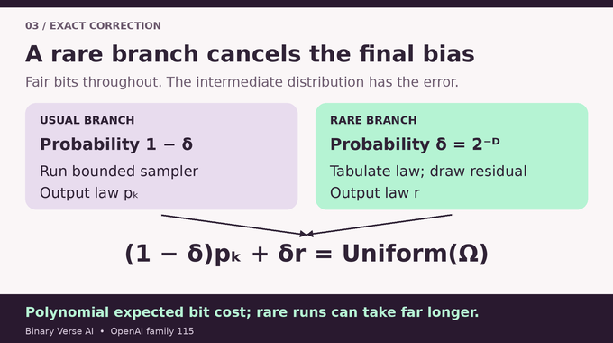
Approximation alone never becomes exact by waiting a predetermined finite time. Section 6 instead tabulates the bounded sampler’s actual output law , including approximate offsets, holds, stopping rules, failed trials, and fallbacks. Finite-state probability propagation avoids enumerating every random-bit string. The tabulation bound is , where .
Set , , and . If , the accuracy and size bounds imply that for every table. The nonnegative residual law is
This is a probability law, distinct from the row-margin vector . Usually the algorithm runs the bounded sampler. Only when all branch bits are zero does it enumerate tables, tabulate the law, and sample the residual using integer weights. That branch occurs with probability . Multiplying its exponential cost by this tiny probability leaves a polynomial contribution to expected cost. Exactness comes from the mixture identity, not rounding away a small error.
11. What the Proof Guarantees and What It Does Not
The theorem covers zeros, highly unequal margins, and varying dimensions. It excludes cell bounds and forbidden positions, or structural zeros. Those appear in a separate approximate-counting companion result. Its deliberately large exponents establish complexity in principle. They do not establish competitive practical runtime or a recommended statistics implementation.
The degenerate cases also have explicit outputs. When the grand total is zero, every entry is zero. With a single row or column, the opposite margins determine every entry. These cases need no mixing argument, and recognizing them directly ensures that the general construction never silently excludes valid inputs at its boundaries.
The distinction between the two runtime guarantees is operational. A bounded approximate run can be stopped on a predetermined schedule with its stated error guarantee. An exact run has a polynomial average cost across random tapes, while a particular execution may take far longer. Almost-sure termination rules out a positive probability of running forever.
The published family 115 formalization scope covers bounded approximate sampling, exact limiting probabilities, feasible halted outputs, almost-sure termination, and expected polynomial bit complexity. The Lean entry point for unconditional sampling exposes the bounded and exact sampling theorems and separately imports counting machinery. This is the published scope, not a claim that we rebuilt the repository or independently audited every dependency. Formalization and independent mathematical review answer different questions, as in our coverage of Lean formal proofs.
The lasting contribution of contingency table sampling here is a constructive chain of guarantees: isolate bounded coordinates, weight completions correctly, prove mixing, implement finite randomness, and cancel the final bias. Read the manuscript alongside this explainer, and follow Binary Verse AI for careful, connected guides to AI-assisted mathematics that make the mechanisms understandable.
What is a 2 × 2 contingency table, and how are its margins fixed?
A 2 × 2 contingency table contains four nonnegative integer entries arranged in two rows and two columns. Fixed margins mean each row and column must retain its prescribed total, even when the individual cell values change.
Is uniform contingency table sampling the same as Fisher’s exact test sampling?
No. Uniform sampling gives every feasible table equal probability. Fisher’s exact test uses a conditional hypergeometric distribution, which generally assigns different probabilities to different tables.
Why is polynomial complexity in the binary length of the margins important?
A margin of size requires only bits to represent for . An algorithm polynomial in could therefore be exponential in input length. The proof instead establishes polynomial dependence on the binary encoding.
Can the exact sampler handle zero or highly unequal row and column margins?
Yes. The theorem allows arbitrary nonnegative integer margins with equal grand totals. It requires no positivity, balance, sparsity, or fixed-dimension assumption.
Does exact uniform sampling guarantee polynomial running time on every execution?
No. Exact uniformity is achieved with polynomial expected bit complexity and almost-sure termination. Exceptionally rare executions involve exhaustive computation.
Does the proof support forbidden cells or structural zeros?
Not in its exact-sampling theorem. The paper considers unrestricted nonnegative entries subject to prescribed margins. Cell bounds and structural zeros belong to a separate companion result concerning approximate counting.
Has OpenAI’s exact contingency table sampling result been formalized in Lean?
OpenAI publishes a Lean formalization covering the exact sampler, almost-sure termination, feasible outputs, uniform probabilities, and expected polynomial bit complexity. This describes the published scope. The existence of Lean code is not independent peer review.