
Imagine a circuit that can conceal its answer by breaking a few carefully chosen gates. The PCP for PPAD Conjecture asks whether that escape route can be closed with almost linear storage overhead. OpenAI’s September 25, 2026 manuscript presents a proof: even an adversarially placed constant fraction of failed constraints cannot prevent polynomial-time recovery of an End-of-Line solution from an acceptable assignment. The achievement combines error tolerance, compact encoding, and universal decoding.
Table of Contents
1. What the PCP for PPAD Conjecture Asks and What the Proof Establishes
Theorem 1.3 in the original research paper fixes positive rational constants and , with and . An input of binary length becomes a generalized circuit of complete binary length satisfying:
Here is a fixed positive integer and a fixed nonnegative integer. Neither depends on the instance. An acceptable rational assignment has polynomial encoding length and satisfies at least a fraction of gates at tolerance . The decoder succeeds for every such assignment.
| Feature | Precise Guarantee |
|---|---|
| Input | Explicit predecessor and successor circuits for End-of-Line. |
| Output size | All gates, connections, indices, auxiliary data, and rational parameter bits count toward . |
| Failures | A fixed positive fraction, with arbitrary locations and violating values. |
| Algorithms | Deterministic polynomial-time construction and decoding. |
| Existence | Every generalized circuit has a polynomially encoded rational assignment satisfying every gate. |
The constants are selected through proof inequalities, rather than presented as simple benchmark tolerances. This is an asymptotic theorem with a finite-witness guarantee. Its quantifiers matter. One fixed construction and one decoder must work across all input lengths and acceptable witnesses. The constants and polynomial bounds are chosen once for all inputs, before inspecting any assignment or its failed gates. An argument covering only random failures would leave the central adversarial guarantee unresolved.
2. End-of-Line: The Search Problem Behind PPAD
PPAD means Polynomial Parity Arguments on Directed Graphs. Its canonical End-of-Line problem describes a potentially exponential graph using short Boolean circuits: a successor and predecessor . An edge is retained when the two descriptions agree. Each vertex has at most one incoming and one outgoing edge. A known source ensures another endpoint exists.
The task is to find a nonzero bit string satisfying:
For a two-bit example, follow the path below. Let the successor fix its terminal vertex and the predecessor fix the source. At the terminal vertex, applying successor then predecessor returns 01 instead of 11, exposing the required mismatch. The unused label 10 can be isolated by making both circuits fix it. Finding an endpoint from a succinct description is different from inspecting an explicitly listed path.
In the toy panel, the first coordinate has four ones and the second also has four ones, so coordinatewise majority reconstructs 11. Merely duplicating an unprotected computation would not establish the theorem: failures could target the common input or its sole extraction wire. The actual construction must protect the decisions that identify a nearby encoding and control how often each physical value is read. That is why redundancy alone is only the beginning of the proof.
3. Why Previous PPAD-Hardness Results Were Not Enough
The classical PCP theorem enables verification of NP witnesses through a few randomized queries. PCP for PPAD asks for analogous robustness within a total search reduction. There is always an answer, and an approximate circuit assignment must still reveal one after some constraints are abandoned.
Rubinstein established constant numerical-error hardness with every gate required to hold. His 2016 work also combined encoded paths, locally evolving computations, and holographic certificates, but left composition unresolved. Constant approximation error alone does not allow an adversary to sacrifice selected gates. Ordinary polynomial-size reductions also need not meet the quasilinear bound.
The manuscript therefore needs two simultaneous guarantees: a fixed failed-gate allowance and almost linear complete storage. Its result concerns that reduction. As with the distinctions discussed in our Weisfeiler–Leman complexity explainer, a hardness classification and a running-time lower bound are separate statements.
4. Generalized Circuits: Two Different Kinds of Error
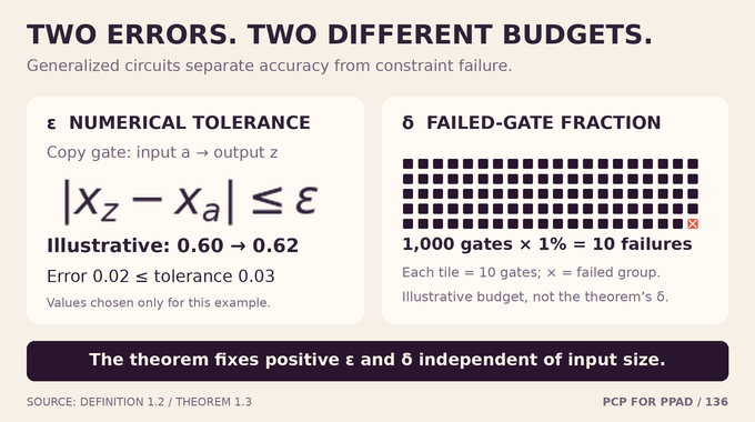
A generalized circuit assigns each node a real value in the unit interval. Gates impose approximate arithmetic or logical relations, and feedback cycles are allowed. For example, an Add gate requires its output to be within of the input sum clipped at one. A Copy gate allows the same numerical tolerance between input and output.
By contrast, limits how many gates may violate their entire relation. Every gate has equal weight. A failed gate may be arbitrarily wrong, but a shared node still has one globally consistent value. With 1,000 gates, a hypothetical one-percent failure allowance permits ten failures. That example is arithmetic illustration, not the theorem’s chosen constant.
Comparison gates use strict input-gap thresholds. Boolean gates use weak thresholds near zero and one. Increasing the tolerance can activate a previously inactive Boolean condition, so the proof cannot casually relax it. These numerical constraints differ from the discrete circuits in our Boolean circuit lower-bound explainer.
5. The Proof Architecture: Encoded Paths and Two Levels of Robust Computation
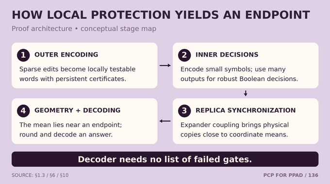
The reduction first makes End-of-Line evolve through sparse edits, then encodes its vertices, then realizes a geometric displacement field using robust local computation. The geometry forces every acceptable assignment to expose an endpoint. Two encoding scales keep this process compact.
| Stage | Stored Object | Required Guarantee |
|---|---|---|
| Outer representation, Sections 2–5 | A vertex word with polylogarithmic-size symbols. | Local tests, neighbor access, and correction with quasilinear storage. |
| Inner port, Sections 7–9 | One binary format for each outer symbol. | Robust Boolean decisions with many designated outputs. |
| Composition, Sections 6 and 10 | Replicated coordinates of an encoded path. | Synchronization and displacement force endpoint recovery. |
Applying a polynomial-size gadget directly to the whole vertex could destroy the size bound. Applying it only to polylogarithmic-size symbols converts that cost into a fixed logarithmic power. The interfaces must also agree on correction radii, query distributions, and physical wire loads.
6. The Sparse Macrograph: Turning Computations into Local Tape Edits
Section 2 replaces a whole circuit transition with a transcript graph whose edges edit at most one tape bit and its occupation bit. Occupation records whether a position has been filled, separately from whether its content is zero. Copy trees bound how many local rules depend on each position.
Two tapes follow four phases: fill the next transcript, erase the old transcript through reverse reconstruction, copy the new transcript into the old tape, and erase the temporary tape. Forward and reverse proposals are checked reciprocally, so retained edges agree in both directions.
A terminal comparison can obstruct a proposed fill. The proposal still writes the computed bit, but its candidate transcript fails validation. This obstruction exposes a predecessor–successor mismatch that decodes to an End-of-Line answer. The construction preserves endpoint information while making transitions locally manageable. A clock extends the represented path without requiring storage of its entire history, a resource distinction also useful in our time–space tradeoff explainer.
7. Outer Encoding: Locally Testable Codes and Persistent Certificates
A single false transcript equation could escape a test that samples equations directly. The outer construction instead represents equation residuals algebraically. On exact codewords, a nonzero remainder differs from zero at a constant fraction of positions, giving local tests a detectable gap.
Systematic square codes provide commuting row and column constraints. Persistent certificates record intermediate products and linear computations. Whole-row or whole-column comparisons detect false certificate identities. Testing all stored components on one fixed neighborhood prevents extra certificates from diluting the gap.
Editing one logical tape position can nevertheless change many encoded entries. Before the edit, the construction prepares each retained array’s finite difference: its new value minus its old value. Newly required increments have lower assigned polynomial degree, so this closure has bounded depth. Fourier work proceeds through small frequency groups with reusable scratch storage. The endpoint representation stays compact even when preparation takes many transitions. This is structured error correction, rather than the observation model of trace reconstruction.
8. The Inner Decision Gadget: One Fixed Port That Tolerates Corrupted Bits
Each outer symbol has bits, with bounded by a fixed power of a logarithm of . The inner encoding maps that symbol into a binary block of length polynomial in . Crucially, its encoding and positive correction radius are fixed before choosing how many symbols a later local computation reads.
Theorem 6.1 then supports Boolean functions of a fixed number of these ports. Sections 7–9 build algebraic path representations, binary tests, and correction procedures. Accuracy is averaged over requests with controlled address density. The theorem does not promise arbitrarily accurate recovery at every individual coordinate.
Many designated wires carry the decision result. This matters because an adversary could otherwise spend a small failure budget on a single answer wire. The inner geometric argument drives feedback near the computation path’s unique sink, where many coordinates reveal the Boolean answer. Separate accounting bounds both corrupted external reads and internal gate failures.
9. Encoded-Path Geometry: Why Approximate Fixed Points Reveal Endpoints
Separated binary vertex words are embedded in four coordinate blocks. Each graph edge becomes a polygon: update the second word block, change a repeated control bit, update the first word block, then reset the control bit. Rounded corners connect these pieces into directed paths and cycles.
The displacement field combines directed motion along a path with attraction toward it, then transitions to a fixed direction farther away. Clipping keeps coordinates inside the box. Outside fixed endpoint neighborhoods, the clipped move has a positive lower bound proportional to a fixed step size. Distances use a norm normalized by encoding length, avoiding dimension-dependent weakening.
Local numerical procedures estimate nearby candidate pieces through validation and corrected bit requests. They allocate a bounded candidate list and estimate its statistics before choosing a numerical winner. This order makes average correction sufficient despite adaptive selection. An extra entrance segment handles the known source, preventing it from serving as the recovered answer.
10. Why Broken Gates Cannot Hide an Answer: The Expander Argument
Every geometric coordinate has many physical replicas. A fixed-degree expander couples them through averaging. Bounded updates and the expander’s spectral gap first force replicas close to their coordinate means, without assuming that Boolean decisions are already correct.
Synchronization bounds deviant reads. Threshold offsets control ambiguous comparisons, while bounded routing load prevents one corrupted value from spoiling too many computations. Gates inside shared decision gadgets, extraction wires, and unused hypothetical branches all enter the accounting. Random tapes describe the analysis, but the printed circuit deterministically enumerates a finite list.
The final contradiction keeps clipping inside the contraction estimate. It does not exchange averaging with nonlinear clipping. Reliable outputs approximate the true field; other satisfied outputs still make bounded steps. If the mean stayed away from every desired endpoint, geometry would require more displacement than the circuit residual permits. The mean must therefore lie near an endpoint. Round its first block, decode the binary ports, then decode the outer word. No list of failed gates is needed. Parameter choices follow a strict order: fix the encoding and geometric requirements, choose correction accuracy and local computations, then select sufficiently small numerical and failure tolerances. Otherwise, improving accuracy could enlarge the very computation whose errors were supposed to have been budgeted.
11. Why the Complete Reduction Remains Quasilinear
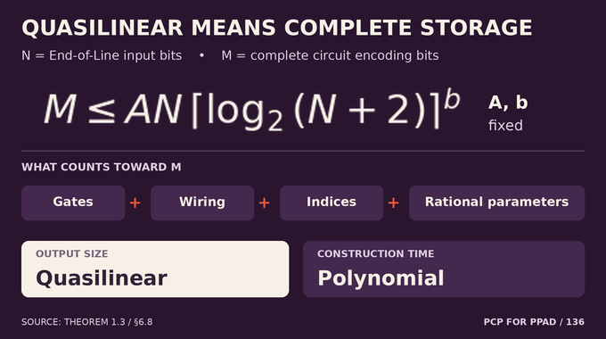
Section 6.8 counts every circuit component, including copied estimators, entire shared invocations, extraction gates, constants, and comparisons on every hypothetical branch. Connection records are explicit. Node identifiers cost logarithmically many bits, and local parameters have polynomial-in- descriptions. These costs increase only the fixed logarithmic exponent.
The construction never enumerates the exponentially large logical graph. All public data and routing records are deterministically constructible in polynomial time. Quasilinear output size alone does not prove quasilinear construction time.
The witness guarantee also matters. Lemma 6.13 uses a continuous cube map, Brouwer’s theorem, and rounding to a fixed rational mesh to establish an assignment satisfying every gate. The mesh denominator depends only on . This proves finite totality, without giving an efficient algorithm to find that assignment. As in approximation-hardness arguments for bin packing, encoding and precision conventions are part of what makes a reduction meaningful.
12. What the Proof Changes for Equilibria and What It Does Not Establish
Section 11 transfers the robust circuit theorem through existing reductions. One consequence concerns two-action polymatrix games of maximum degree three: finding a profile where all but a fixed fraction of players have regret below a fixed threshold is PPAD-hard. Other consequences cover relative approximate bimatrix equilibria, course allocation, specified market equilibria, and stationary equilibria in discounted games. Their approximation definitions differ. The paper also tracks rational witness sizes and decoder costs when transferring hardness. These details specify which finite computational problem is hard, rather than simply attaching the same conclusion to every notion of approximate equilibrium.
These are worst-case hardness results, not measured solver performance or a claim that every equilibrium instance is difficult. Stronger time lower bounds can retain ETH for PPAD. That assumption should not be conflated with ordinary SAT-based ETH, discussed in our Exponential Time Hypothesis explainer.
Verification scope is equally specific. OpenAI’s mathematics release announcement describes AI-produced research and accompanying formalizations. The supporting generalized-circuit Lean development proves endpoint existence and supporting smoothing, perturbation, and mesh facts. Its header explicitly leaves simultaneous totality and the uniform quasilinear reduction, soundness, algorithm realization, and complexity bounds unproved. Defining a goal proposition does not prove it. The manuscript’s theorem and the available formalization therefore have different scopes.
The PCP for PPAD Conjecture centers on a demanding combination: compact storage, fixed numerical slack, and decoding that survives adversarial constraint failures. The proof’s lasting idea is how local redundancy becomes a global endpoint guarantee. Follow Binary Verse AI for careful research explainers that connect theorem statements to the mechanisms, assumptions, and verification evidence behind them.
What does PPAD stand for, and what problem does it study?
PPAD stands for Polynomial Parity Arguments on Directed Graphs. It is a complexity class of total search problems, including End-of-Line, where a directed graph’s endpoint structure guarantees that a required solution exists.
How does the PCP-for-PPAD conjecture differ from the classical PCP theorem?
The classical PCP theorem concerns efficient verification of NP witnesses through limited randomized access. PCP-for-PPAD seeks analogous robustness for total search reductions, allowing a positive fraction of approximate circuit constraints to fail while retaining endpoint recovery.
Why was the PCP-for-PPAD conjecture difficult to prove?
Earlier constructions established hardness under numerical approximation but did not simultaneously guarantee quasilinear complete reduction size and recovery despite an arbitrary constant fraction of violated constraints. The proof must compose robust local computation without losing either guarantee.
How can the reduction recover an answer when some circuit gates fail?
The proof combines encoded representations, local correction, redundant decision outputs, and expander-based synchronization. Its clipped-displacement argument forces the mean geometric state near a recoverable endpoint despite a bounded fraction of failed gates. The decoder need not know which gates failed.
What makes the PCP-for-PPAD reduction quasilinear?
An End-of-Line instance of binary length becomes a generalized circuit whose complete encoding requires only bits. This counts wiring, indices, auxiliary gates, and rational parameter bits. It is a size bound; the theorem separately guarantees polynomial construction time.
Does OpenAI’s proof provide explicit values of ε and δ?
The main theorem establishes fixed positive rational constants independent of input size, with and . They are selected through proof inequalities, rather than supplied as simple numerical values for directly benchmarking an implementation.
Does the proof settle Nash equilibrium hardness, and has it been formalized in Lean?
The paper derives specific PPAD-hardness consequences for approximate equilibrium problems through existing reductions. Additional time lower bounds can still require ETH for PPAD. The available Lean development contains endpoint-existence and supporting circuit and mesh results, but explicitly leaves the uniform quasilinear theorem and simultaneous circuit totality unproved. It is not a full formal verification of Theorem 1.3.