
A function can have a derivative everywhere without that derivative varying continuously. That gap is the central issue in higher-dimensional infinity Laplacian regularity. OpenAI’s October 4, 2026 manuscript proves that bounded infinity-harmonic functions in dimensions have uniformly Hölder-continuous gradients on interior balls. The exponent is positive and dimension-dependent, but unspecified. The proof converts qualitative flatness into a power law by showing that a hypothetical failure would generate an entire nonaffine limit that its Liouville theorem forbids.
Table of Contents
1. Infinity Laplacian Regularity: The Higher-Dimensional Problem
The underlying extension problem asks for a function that minimizes its largest local slope. An absolute minimizer must do this on every relatively compact open subdomain, against Lipschitz competitors with identical boundary values. Minimizing globally alone does not capture this local requirement.
The original regularity manuscript supplies the theorem and proof examined here. OpenAI’s mathematics release announcement provides attribution and release context. Its statement that many proofs have Lean formalizations does not establish formal verification of this particular theorem. The supplied PDF presents an analytic proof, not a numerical performance benchmark.
| Item | Verified Scope |
|---|---|
| Solutions | Bounded, continuous infinity-harmonic functions on . |
| Dimension | Every integer . |
| Conclusion | , with . |
| Uniformity | Constants depend only on dimension. The bound scales with oscillation. |
| Limits | No explicit exponent, optimal endpoint, or boundary estimate. |
2. The Infinity Laplace Equation And Its Degenerate Geometry
Here is the gradient, the Hessian, and first and second partial derivatives. At a smooth point with nonzero gradient, the equation controls curvature along that gradient. It does not control every second derivative independently. At zero gradient, the unnormalized operator vanishes regardless of the Hessian.
Because solutions need not possess classical second derivatives, the paper uses viscosity tests. If a smooth function touches the solution from above, its infinity Laplacian must be nonnegative. A lower touching test must give a nonpositive value. Tests with zero gradient remain included. Infinity Laplacian viscosity solutions therefore satisfy a precise comparison rule even where writing a classical Hessian for the solution is impossible.
3. Why Earlier Differentiability Results Were Not Enough
Earlier infinity harmonic regularity theory established that infinitesimal blow-ups at a fixed point are affine. In the plane, Savin proved gradient continuity, followed by the Evans–Savin interior Hölder estimate. The Evans–Smart differentiability theorem subsequently supplied a unique derivative at every point in every dimension.
These conclusions occupy different levels. An affine subsequential blow-up identifies a possible tangent plane. Differentiability makes its slope unique. Gradient continuity compares slopes at neighboring points, while a uniform Hölder estimate supplies one quantitative comparison across a whole normalized family.
The manuscript also cites 2026 planar endpoint work, including a restricted theorem by Brustad and an unrestricted local statement by Xu that separately leaves a universal endpoint norm estimate open. Those planar developments should not be confused with this paper’s higher-dimensional uniform estimate.
4. OpenAI’s Uniform Interior C¹,α Theorem Explained
Theorem 1.1 assumes is bounded and infinity-harmonic, with and . There exist and ] depending only on dimension such that
Oscillation means supremum minus infimum. The Hölder seminorm measures the worst gradient difference divided by the distance raised to the exponent:
For infinity-harmonic functions, this regularity means more than smooth-looking graphs. After normalizing oscillation, one constant controls both gradient size and gradient variation. Rescaling around an interior point gives, with an enlarged dimensional constant,
The larger closed ball must lie inside the domain. Continuity bounds the function there, so the estimate applies locally and proves Corollary 1.2: every continuous infinity-harmonic function on an open domain in these dimensions is locally continuously differentiable.
Uniformity matters because the estimate is shared by all solutions satisfying the hypotheses, rather than fitted separately to each function. A smaller oscillation proportionally reduces the allowed gradient size and variation. The distance from the boundary enters through rescaling, explaining why an interior estimate becomes weaker as the available surrounding ball shrinks.
5. Aronsson’s Example And The One-Third Exponent
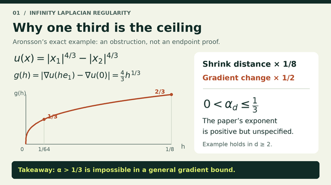
Aronsson’s infinity-harmonic example is independent of the remaining coordinates. Along the first coordinate axis, its gradient obeys
For an exponent larger than one third, dividing by makes the Hölder quotient diverge as . No general gradient estimate with a larger exponent can hold. The example rules out excessive regularity, but does not prove that every solution attains the one-third endpoint.
Away from the coordinate axes, the two nonzero contributions and cancel. On the axes, second derivatives can be singular, so the solution must be interpreted through viscosity tests. This is why the result concerns first derivatives with quantitative continuity rather than general second-order smoothness.
For a concrete comparison, taking gives a gradient difference of , while gives . Shrinking the displacement by a factor of eight only halves the gradient difference. That exact scaling makes the one-third obstruction visible without relying on a plotted approximation, and persists when the example is extended into higher dimensions.
6. The Linear Lift And Three-Point Flatness Estimate
The proof first normalizes oscillation and adjoins one coordinate: . Lemma 2.1 verifies viscosity preservation, including tests whose original horizontal gradient vanishes. The added component is exactly one, preventing accurate fitted slopes from collapsing to zero.
Proposition 2.5 then addresses a subtle mismatch of scales. For uniformly Lipschitz infinity-harmonic functions approaching affine functions on the unit ball,
The numerator is the midpoint defect. Crucially, the estimate includes arbitrarily short endpoint separations. Ordinary uniform convergence would control the numerator, but division by a much smaller separation could destroy that control.
The proof combines a three-variable viscosity comparison with a concave separation penalty. This transfers affine approximation from a larger observation scale to much smaller scales, yielding uniform qualitative flatness across solutions and centers. Pointwise affine blow-ups alone would not provide that uniformity.
7. Thin Cylinders And The Search For Power-Law Flatness
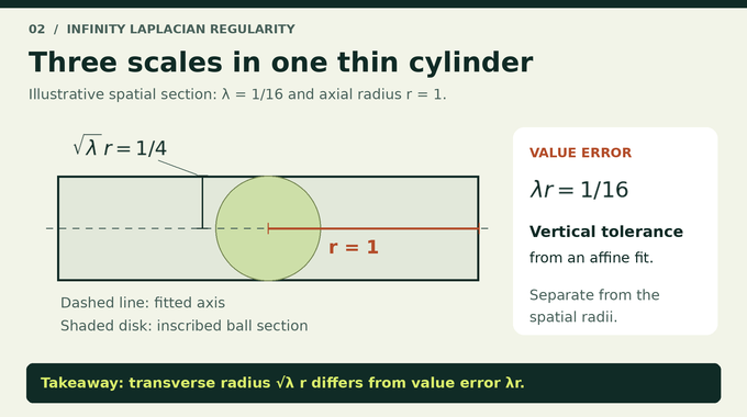
A cylinder fit approximates the lifted function by an affine function whose slope sets the axis. Its axial radius is , transverse radius , and allowed function-value error . These are different geometric and vertical scales.
The modulus takes the worst fitting obstruction across normalized solutions, interior centers, and radii at most times the distance to the working boundary. Technically it uses the supremum of bad parameters, since goodness need not be monotone in . Lemma 3.2 proves . Proposition 3.3 seeks the stronger bound for some positive .
The cylinder geometry encodes the degeneracy. Longitudinal and transverse perturbations are not treated on the same scale. Comparing fits on their common inscribed balls controls slope directions, while comparison along a shared axial segment gives stronger control of slope magnitudes. Both estimates are needed: after rescaling, an error harmless in the original coordinates might otherwise become unbounded.
8. When Power Decay Fails: Constructing The Nonaffine Limit
Suppose every power bound fails. Lemma 3.4 selects small bad scales and parameters . The selected parameter fails at its center, while succeeds uniformly at nearby centers and every fixed multiple of that scale, eventually along the sequence.
Comparisons of overlapping cylinders control both slope directions and slope magnitudes. After aligning the central axis, the proof stretches transverse coordinates and magnifies the residual from its affine fit. Those comparisons give local bounds and equicontinuity, allowing a subsequence to converge on the whole enlarged space.
The variable is the axial coordinate, not physical evolution time. Before passage to the limit, the final component of the test direction is . Viscosity stability gives the displayed limiting equation. If the limit were affine, pulling its fit back would improve the deliberately failed cylinder fit. Proposition 3.6 therefore retains nonaffinity.
The bad-scale selection does two jobs simultaneously. Failure at the distinguished cylinder preserves an obstruction, while nearby successful fits prevent the rescaled functions from becoming uncontrollable. Taking an arbitrary sequence of shrinking radii would not ensure both properties. This is the bridge between the failure of a quantitative rate and a globally defined limiting object.
9. The Liouville Theorem: Why The Limit Must Be Affine
Theorem 3.1 applies to entire continuous viscosity solutions of the limiting equation in , for . At every center and radius, it additionally requires a uniform fit:
One finite works everywhere, although and may vary. The paper writes , which makes its frame changes transparent. The horizontal slope also determines the box’s shear. These hypotheses force affinity, not the equation alone.
The constructed limit inherits precisely these estimates. Comparing fits supplies compactness after recentering and subquadratic spatial growth. That growth also confines the quadratic optimizers used next. This Liouville argument therefore depends on a carefully restricted class, rather than an unrestricted assertion about all entire solutions.
The all-scale hypothesis is especially important at large radii. Local fits alone would not constrain behavior at infinity strongly enough for the global envelope argument. Changes of frame translate, rescale, shear, and subtract a compatible affine function while preserving the class. They let the proof normalize a chosen fit without losing its global assumptions.
10. Quadratic Envelopes And The Extremal Horizontal Defect
The forward envelope maximizes . The backward envelope minimizes . Their difference quotients relative to are nondecreasing in length, with a common small-length limit that can initially be minus infinity.
To preserve an obstruction to affinity, Section 5 uses a horizontal Jensen defect: the weighted average of values minus the value at their spatial mean. Recentring near-extremal configurations maximizes defect divided by root mean square radius, producing a positive extremal constant .
The barycentric envelope maximizes those weighted averages after subtracting variance divided by . The extremal defect bound yields . Setting and subtracting produces a subsolution touching at positive time. At contact, the unshifted envelope gap remains positive. The viscosity argument works because the variance penalty is affine along the specific testing directions, so it contributes no second variation there.
For intuition, an equal-weight two-point configuration compares the mean of two values with the value at their midpoint. Every affine function gives zero defect. The proof allows arbitrary finite configurations, so it can select an extremal obstruction and pass it through compactness. Subquadratic growth prevents distant configurations from escaping the quadratic penalty. The quadratic envelopes play a different role: their slopes measure change across the axial coordinate. Agreement as lengths shrink does not itself make them constant at larger lengths. Achieving that stronger equality is the purpose of the final localization argument.
11. Contact Propagation, Localization, And Final Rigidity
Sections 6–7 turn that contact into an enduring configuration. Forward optimizers for and backward optimizers for define two discrete steps. A fair choice creates a drift inequality controlling the accumulated squared discrepancies between their velocities and one common reference velocity. Fitted frame changes preserve this control.
The resulting stopped walks supply contacts at shrinking positive times. More is needed than a sequence of unrelated contacts: Proposition 7.1 localizes infinitely many fitted frames around one terminal point at time zero, where the common small-length envelope slope is finite.
Normalizing at those contacts makes every fixed envelope length correspond to a shrinking length at that same terminal point. Subtracting two normalized slopes cancels the affine correction. The final compact limit consequently has equal forward and backward slopes, constant at every positive length.
Lemma 8.1 uses quadratic comparison to identify one common equality velocity and squeeze the solution to an affine function. Yet the normalized positive barycentric gap survives. An affine function has zero such gap, giving the contradiction that proves rigidity.
The random choice is a proof device. Its axial coordinate can step forward or backward, so the construction is not a monotone trajectory of contacts. Stopping and expectation estimates control the walk, while a joint limit retains the terminal point together with marks at smaller scales. Keeping one endpoint is essential: finite slope information at unrelated points would not identify a common final limit. Likewise, finiteness must be proved, because the general envelope lemma permits a slope of minus infinity. Once a finite common slope is secured, cancellation of the frame corrections makes fixed-length slope differences vanish. The positive normalized envelope gap remains available to contradict affinity.
12. From Power Decay To Hölder Gradients: The Final Step And Remaining Limits
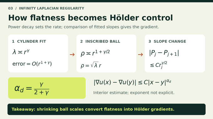
The contradiction establishes power decay. With , an inscribed ball has radius , while fitting error is of order . Successive slope differences are , so the fitted slopes converge uniformly. Matching these scales gives
The limiting slope yields a uniform Taylor remainder of order . Comparing expansions from two neighboring centers then gives the gradient Hölder bound. This completes the infinity Laplace equation regularity proof and explains why qualitative flatness alone was insufficient.
Concretely, subtracting two Taylor expansions eliminates the function values and isolates the difference between their fitted linear parts. Evaluating along each unit direction controls every component of that difference. The resulting estimate is therefore a statement about the whole gradient, despite the original equation controlling only curvature along one direction.
| Established | Still Outside This Result |
|---|---|
| Uniform interior gradient control | An explicit optimal exponent or endpoint estimate. |
| Local continuously differentiable solutions | General second derivatives or boundary regularity. |
| A compactness-based analytic argument | A numerical convergence rate or solver benchmark. |
Infinity Laplacian regularity here means a uniform interior theorem, with neither the optimal higher-dimensional endpoint nor boundary estimates established. For related PDE research, explore Binary Verse AI’s explainers on Lane–Emden, local smoothing, hot spots, Navier–Stokes, Vlasov–Maxwell, and strong cosmic censorship. Follow Binary Verse AI for careful explanations connecting theorem statements to the mechanisms that prove them.
Are infinity-harmonic functions continuously differentiable in dimensions three and higher?
The October 2026 paper proves that infinity-harmonic functions are locally in every dimension . More strongly, it establishes an interior Hölder estimate for their gradients with a positive dimension-dependent exponent.
What does C¹,α regularity mean for the infinity Laplace equation?
It means the solution has continuous first derivatives and its gradient satisfies a bound of the form . The theorem provides uniform control on interior balls, with constants depending only on dimension after normalization.
Wasn’t differentiability of infinity-harmonic functions already proved?
Yes. Evans and Smart established everywhere differentiability in every dimension. The new proof establishes the stronger property that gradients vary Hölder-continuously, with uniform quantitative control.
Why is the infinity Laplace equation difficult to analyze?
The unnormalized operator involves second derivatives only in the direction of . This degeneracy prevents direct application of standard uniformly elliptic regularity methods and makes control of the entire gradient difficult.
Does the proof establish the optimal Hölder exponent 1/3?
No. It produces an unspecified positive exponent . Aronsson’s example shows that a larger exponent is impossible in general, but the higher-dimensional optimal endpoint is not established by this manuscript.
Why does the proof need a Liouville theorem?
The argument assumes uniform power-law flatness fails and constructs a nonaffine entire solution of a limiting equation. The Liouville theorem shows that every such solution satisfying the inherited sheared-box estimates must be affine, producing a contradiction.
Does the result prove C² regularity or regularity up to the boundary?
No. The theorem concerns interior estimates. It makes no boundary regularity claim, and Aronsson’s example demonstrates why general second-order smoothness cannot be expected.