
A black hole can have a boundary across which distances remain continuous while the mathematical machinery for transporting vectors becomes too singular. That gap is the target of OpenAI’s strong cosmic censorship proof near Kerr. Its September 23, 2026 manuscript presents a precise result: near each fixed rotating, subextremal Kerr bridge, data allowing a future continuous extension with a locally square-integrable weak connection form a meagre set. The conclusion concerns generic nearby vacuum data, not every black hole or every continuous extension. The decisive argument combines exact gravitational wave packets, controlled nonlinear evolution, and averaged parallel transport.
Table of Contents
1. Strong Cosmic Censorship: The Problem of Predictability in General Relativity
General relativity starts with initial data: a spatial metric describing geometry and a second fundamental form describing how that slice sits in spacetime. They must satisfy Einstein’s constraint equations. Their maximal globally hyperbolic development, abbreviated MGHD, is the largest development uniquely determined by those data within the globally hyperbolic class.
“Maximal” does not automatically mean no larger spacetime exists. An extension embeds the MGHD isometrically as a proper open region of a larger manifold. The strong cosmic censorship conjecture asks whether generic data prevent such continuation, with the allowed regularity specified. Changing that regularity changes the question.
| Property | Precise Scope |
|---|---|
| Background | Each fixed Kerr bridge with and . |
| Initial data | Smooth, complete, two-ended vacuum data near that bridge. No symmetry imposed. |
| Forbidden extension | Continuous, nondegenerate metric in , reached by a future timelike exit. |
| Genericity | Extendible data are meagre. Inextendible data contain a residual subset. |
| Smallness | Only the tenth weighted seminorm must be small. The topology tests all finite orders. |
| Beyond the boundary | Neither vacuum equations nor global hyperbolicity are required outside the embedded development. |
The manuscript’s Definition 1.1 and Theorem 1.2 define both the geometric setting and the excluded extension class. Our guide to AI mathematical proofs explains why identifying the exact theorem is the starting point for evaluating model-generated research.
2. Why the Kerr Cauchy Horizon Makes the Problem Difficult
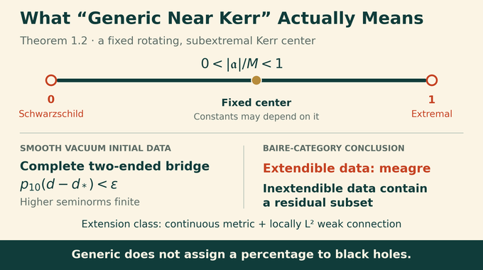
Kerr spacetime describes a rotating vacuum black hole. Write for mass and for its signed rotation parameter. The condition selects rotation strictly between the nonrotating and extremal cases. The initial hypersurface is the complete two-ended bridge through the bifurcation sphere, with topology . It has two asymptotically flat ends.
Inside exact Kerr lies an inner Cauchy horizon. Beyond it, the globally hyperbolic development admits smooth continuation, but the original initial data no longer determine the continuation through global hyperbolicity. Exact Kerr therefore supplies an exceptionally orderly example that a genericity theorem must allow.
Perturbations make that order precarious. Radiation approaching the inner horizon undergoes blueshift, motivating Cauchy horizon instability. Yet “the disturbance grows” is only a physical guide. A proof must identify which geometric quantity obstructs which extension class, and must address arbitrary candidate exits. Ruling out continuation through one carefully chosen horizon patch would leave a route around the argument.
3. The Previous Barrier: Continuous Extensions and Weak Null Singularities
A weak null singularity can preserve a continuous metric while losing stronger regularity. In their Kerr interior stability theorem, Dafermos and Luk proved continuous extendibility across a nontrivial Cauchy-horizon portion for appropriately controlled interior data. Those assumptions matter: this is not an assertion about unrestricted collapse.
The manuscript also builds on work excluding smoother continuations. But excluding twice-differentiable or continuously differentiable extensions does not exclude a weaker Sobolev extension. On a common smooth chart, the relevant permitted classes satisfy:
| Metric Class | What It Permits |
|---|---|
| Continuous derivatives through second order. This is the smallest displayed extension class. | |
| Continuous first derivatives, allowing more candidate continuations. | |
| Continuity plus locally square-integrable weak first derivatives. This paper targets this larger class. | |
| alone | Continuity without the weak-derivative requirement. The theorem does not exclude all such extensions. |
The paper’s companion manuscripts supply comparison geometry and perturbation machinery. Their headline inextendibility theorems are not premises of this proof. The new work must reach the weaker connection threshold directly.
4. What the OpenAI Proof Actually Establishes: Theorem 1.2
Fix the Kerr datum . The paper measures differences using weighted seminorms : suprema of derivatives through order , with radial weights controlling decay along both ends. Metric differences carry weights increasing from one power of radius, while differences in start at two. The neighborhood is:
Here is the specified smooth vacuum constraint-data space. Theorem 1.2 says that, for a sufficiently small positive depending on the fixed Kerr center, data in this neighborhood whose full MGHD admits the defined future extension form a meagre set. Inextendible data consequently contain a residual subset in the weighted smooth topology.
Only must be small. Higher derivatives must have finite weighted seminorms, and every finite order remains available for testing open sets. No extra fixed-charge or parity condition is imposed. The theorem is not restricted to a separately constructed interior fragment.
OpenAI describes its October mathematics release, which includes this manuscript, as results produced by an internal frontier model. As checked on October 22, 2026, its formalization catalogue contains no entry for this Kerr result. The repository’s verification notice acknowledges varying verification stages. Publication of this preprint does not establish independent mathematical acceptance. Discovery and formal verification remain separate tasks, as our Fermat formalization explainer illustrates.
5. Why a Square-Integrable Connection Is the Critical Threshold
The metric measures lengths and causal relations. Its connection describes differentiation and parallel transport. Christoffel coefficients combine first derivatives of metric components with the inverse metric. For rough metrics, these derivatives must be understood weakly, as distributions.
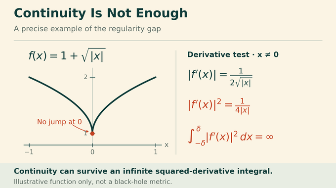
The notation means that components and their first weak derivatives are square-integrable on compactly contained coordinate regions. For a continuous, nondegenerate metric, local bounds on the metric and its inverse make this equivalent to locally weak Christoffel coefficients. A derivative existing almost everywhere is not, by itself, enough.
Why this threshold? Products of connection coefficients are locally integrable, while derivatives can be interpreted distributionally. That supports the weak-curvature framework discussed in the paper. Continuity alone offers no comparable derivative control.
There is a catch: a volume integral controlling the connection does not provide a trace along any prescribed curve. A singular function can behave badly on a thin set without violating its volume bound. Thus the proof cannot simply pick one observer, integrate the extension connection along that trajectory, and declare victory.
6. From an Arbitrary Future Exit to a Family of Timelike Geodesics
Section 3 starts with any extension satisfying the definition and a future-directed timelike curve reaching its boundary. Using compact causal diamonds inside the original globally hyperbolic spacetime, it constructs a local Lipschitz first-exit graph. In coordinates, that graph records where nearby vertical timelike segments first leave the original region.
Averaging connection mass near this graph then produces a positive-measure family of timelike geodesics with finite future proper lifetimes in the full development. Their endpoints and velocities have controlled chart descriptions. All geodesic equations are solved in the smooth original spacetime, not across the rough boundary.
Hamiltonian section volume preserves the relevant measure of positions and momenta. This matters when the proof later transports the observer family to late observation surfaces. Position volume alone would lose the momentum information needed for that comparison.
The comparison geometry classifies finite-lifetime first runout into branches and corners. Corner seeds form a measure-zero set, so a positive family survives on a branch. First comparison runout is not automatically the endpoint of the full geodesic. Keeping those events distinct lets the argument cover actual future exits without assuming their location in advance.
7. Constructing Exact Vacuum Wave Packets Near Kerr
Next comes a deliberately engineered gravitational disturbance. Section 4 launches a finite, oscillatory wave packet whose backward null rays reach a selected exterior end. A launch bump covers the whole observation footprint, ensuring the eventual test does not depend on hitting one privileged point.
A linearized wave is insufficient. The perturbed metric and second fundamental form must satisfy the nonlinear vacuum constraints exactly, or their evolution would not test the theorem’s data space. A support-preserving correction repairs the constraint defect while retaining a decaying exterior tail.
The resulting complete data agree with the background on the other end, the connecting region, and an expanding protected ball. The correction tail and any charge change remain part of the new datum. Nothing is silently replaced by exact Kerr at infinity.
For any chosen finite seminorm order, sufficiently late packets approach the background in that seminorm. This gives freedom to perturb inside an arbitrary prescribed open neighborhood. Readers familiar with physics-informed neural networks should distinguish a small numerical residual from exact constraint satisfaction. Here the correction makes the experiment an admissible test of vacuum general relativity.
8. The Double-Null Nonlinear Comparison: Controlling the Error
Double-null coordinates use two optical coordinates, and , adapted to intersecting lightlike hypersurfaces. Along the chosen branch, one remains bounded while the other grows. Let be a late value of that growing coordinate and the fixed lapse decay rate. The packet amplitude is:
Near observation, the lapse coefficient is comparable to . The packet amplitude therefore decays more slowly than its square root. That choice leaves a detectable signal, but makes nonlinear comparison more demanding than simply evolving an infinitesimal wave.
An optical coordinate change produces a double-null comparison template. The actual vacuum solution must track this template through the finite slab. Theorem 5.1 controls their difference by at every preassigned finite derivative order: the error divided by the signal scale tends to zero.
The mechanism retains lapse factors that compensate losses in angular elliptic estimates. High-derivative bounds and a quadratic low-order error estimate feed an interpolation argument. The resulting improvement closes a bootstrap assumption, while finite-domain restarting ensures the solution actually reaches the observation region.
The experiment’s output is a controlled vacuum solution on the required finite domain. As in our Navier–Stokes proof analysis, gauge choices, domains, and quantitative hypotheses determine what the conclusion means. Restart times need not remain uniform as grows.
9. The Curvature Signal and Matched Observation States
Curvature enters through a two-by-two null-angular block, denoted . Its entries pair the curvature operator applied to the growing null direction and an angular direction with those directions again. This measures a selected geometric response, rather than an unspecified scalar called “the curvature.”
Precisely, , with labeling angular directions and the curvature operator. Let denote the exact perturbed metric and the packet’s oscillation frequency. The frequency grows with , at a rate chosen after the required derivative orders are fixed. Proposition 6.2 gives, throughout the observation patch wherever , the bound:
The cosine condition excludes phase zeros. It occupies two thirds of each complete oscillation period, leaving ample observation parameters. The proof does not assume the background curvature is small. It controls a difference on an entire footprint.
The developments are compared at identical numerical terminal positions and covariant momenta on a transverse section. The appropriate future unit tangent is reconstructed separately for each metric. Matching positions without momenta would compare different observer families and undermine the measure argument.
Canonical volume preservation ensures that observers good for both possible extensions still overlap. Smooth Cauchy stability preserves a slightly weaker signal in nearby data for each fixed finite experiment. No continuity of maximal geodesic lifetime is needed.
10. Averaged Holonomy: How the Proof Rules Out Weak Extensions
Parallel-transport a vector around a small closed loop. Curvature generally prevents it from returning unchanged. This mismatch is holonomy. Shrinking loops extracts curvature from transport, giving the proof a geometric bridge between the smooth interior and a hypothetical rough extension.
The obstacle is still the missing connection trace on individual curves. Section 7 averages over observation positions and bounded momentum labels before closing the transport estimate. The extension’s connection bound then controls most sampled loops, apart from an exceptional parameter set whose measure vanishes.
A stopping rule keeps each loop inside its selected ambient chart and prevents uncontrolled frame growth. Finite interpolation in loop size extracts the desired curvature coefficient with an bound on the surviving observations. This ordering is essential: averaging comes before the chart estimate is closed.
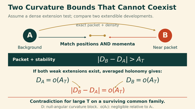
Now suppose two compared developments both admit the prescribed extension witnesses. On a positive-measure overlap, holonomy would make each curvature block smaller than the packet scale. Their difference must then also be smaller than that scale. Yet the persisted packet construction forces the difference to exceed .
The contradiction concerns two extendible developments. It does not assume one globally preferred boundary chart or attach well-defined rough transport to a handpicked curve. Those are precisely the shortcuts that the weaker connection regularity disallows.
11. The Baire-Category Conclusion: What Is Generic and What Remains Outside the Proof
Possible extensions are covered by countably many tests encoding finite chart bounds and large relative observer families. If one test were dense in a nonempty open data set, the construction would supply an extendible background, a nearby packet experiment, and another extendible datum close enough to preserve its finite observations. The curvature contradiction defeats that density.
Each test is therefore nowhere dense. Their countable union is meagre, and its complement contains a residual set of future-inextendible data. This is Baire-category genericity. It assigns no numerical probability to an astrophysical black hole and does not assert that inextendibility is open.
The boundaries are substantial: the theorem does not cover Schwarzschild, extremal Kerr, arbitrary far-from-Kerr data, or every gravitational-collapse configuration. Constants may depend on the fixed Kerr center, without uniform estimates toward either excluded rotation endpoint. Merely continuous extensions remain outside its obstruction. As with the restricted scope in our Hodge conjecture explainer, dropping a hypothesis changes the result.
For AI researchers, the practical lesson is to audit the theorem, dependencies, and verification status together. For developers evaluating scientific reasoning, exact constraints, approximation errors, and observation matching provide concrete checkpoints. Strong cosmic censorship here turns on a specific regularity threshold and a carefully measured contradiction. Follow Binary Verse AI for source-led proof explanations, including our Bose–Einstein condensation analysis, that keep the mechanism and its limits visible.
What is strong cosmic censorship in general relativity?
It asks whether generic initial data determine a maximal globally hyperbolic spacetime that cannot be extended at a specified regularity. The OpenAI manuscript studies future extensions near each fixed rotating, subextremal Kerr vacuum bridge.
Why is the Kerr Cauchy horizon a problem for determinism?
The exact Kerr solution has an inner Cauchy horizon across which its globally hyperbolic development can be extended. Beyond that horizon, the original initial data no longer determine the continuation through global hyperbolicity. The question is whether sufficiently regular extensions survive generic perturbations.
Does continuous extendibility contradict the OpenAI proof?
No. A metric can remain continuous while its weak connection fails to be locally square-integrable. The manuscript generically excludes extensions satisfying both continuity and the specified weak-derivative condition, not all continuous extensions.
What does a square-integrable connection mean?
It means that the weak Christoffel coefficients belong locally to . For the continuous, nondegenerate metrics considered in the manuscript, this is equivalent to regularity in smooth coordinate charts. The derivatives are distributional derivatives.
How does the OpenAI proof establish inextendibility?
It constructs exact vacuum perturbations producing a controlled curvature difference. Averaged holonomy estimates would force that difference to be smaller if both compared developments admitted the specified weak extensions. The contradiction makes each countable extension test nowhere dense.
What does generic mean in the theorem?
Data admitting the specified extension form a meagre set, while inextendible data contain a residual subset of the weighted smooth neighborhood. This is Baire-category genericity, not a numerical probability statement or a claim that inextendibility is open.
Does the proof establish strong cosmic censorship for every black hole?
No. The manuscript concerns smooth vacuum data near each fixed rotating, subextremal Kerr bridge. It does not establish the corresponding statement for Schwarzschild, extremal Kerr, arbitrary far-from-Kerr data, or every gravitational-collapse configuration.