
Finding one valid assignment can be easy while estimating how many assignments exist remains stubbornly hard. A four-edge bipartite square captures the difference: selecting one perfect matching answers feasibility, but the graph has two. Scale up the constraints, and enumeration quickly becomes the wrong tool.
Counting Common Bases of Two Matroids asks for the number of subsets satisfying two matroid basis conditions simultaneously. OpenAI’s September 23, 2026 preprint presents a fully polynomial randomized approximation scheme, or FPRAS, for arbitrary equal-rank matroids supplied through exact independence oracles. It promises a relative-error estimate with controlled failure probability and polynomial work on every execution. The advance concerns a universal algorithmic guarantee, rather than a demonstrated application speedup.
Released in OpenAI’s October mathematics collection, the proof combines algebraic inequalities, carefully balanced defect states, and a selective analysis of a random walk. Its most revealing move is deciding exactly which fluctuations need control.
Table of Contents
01. What Does Counting Common Bases of Two Matroids Mean?
A matroid describes independence on a finite ground set. The empty set is independent, subsets of independent sets remain independent, and augmentation lets a smaller independent set acquire some element from a larger one while preserving independence. Rank is the largest independent subset size. A basis is a maximal independent set, and every basis has the matroid’s rank.
Let and have rank on labeled elements. Write for the bases of a matroid. The target is:
For the square example, the ground elements are edges. One partition matroid permits at most one edge per left vertex, the other at most one per right vertex. Their rank-two common bases are the two perfect matchings. The paper’s Theorem 1.1 estimates this count with any specified rational error and confidence tolerances.
01.1. Counting Common Bases of Two Matroids: Key Facts
| Question | Verified Scope |
|---|---|
| Input | Two equal-rank matroids on an explicitly enumerated ground set. |
| Access | Fixed, exact independence oracles. No matrix representation required. |
| Output | Nonnegative rational estimate with relative error at most , except with probability at most . |
| Resources | Polynomial oracle calls and other bit operations on every execution. |
| Status | Released preprint with a linked Lean development. Practical speedups are not demonstrated. |
02. Why Is Counting Common Bases Harder Than Matroid Intersection?
Matroid intersection counting starts where optimization stops. Matroid intersection finds a largest set independent in both matroids in deterministic polynomial time. For equal ranks, its size tells us whether a common basis exists. One witness, however, says little about the size of the entire feasible family.
Bipartite perfect matchings explain the complexity gap. Their exact count is the permanent of the graph’s zero-one adjacency matrix, a classical #P-complete counting problem. Thus general exact common-basis counting contains #P-hard instances. An approximation theorem does not turn that exact problem into a polynomial-time one.
For bipartite graphs, a permanent FPRAS already exists through Jerrum, Sinclair, and Vigoda. The new target is every pair of oracle matroids, including pairs that lack the representation or stability assumptions exploited by specialized methods. The square is an illustration of the reduction, not evidence that this toy instance needs sophisticated machinery.
Readers of our Subset Sum algorithm analysis will recognize the editorial lesson: specify whether a theorem decides existence, constructs a witness, or estimates a count. Those outputs answer different questions.
03. The Previous Barrier: Why Existing Approximation Algorithms Fell Short
Anari, Oveis Gharan, and Vinzant’s earlier deterministic approximation result achieved a factor in polynomial time. That factor can grow exponentially with rank. It is not the same as demanding, say, five-percent relative error.
Their relative-approximation approach retained exponential rank dependence in its runtime. When rank is logarithmic in ground-set size, that dependence becomes polynomial. When rank grows freely with the input, it remains a barrier. Removing it is the specific promise behind a matroid intersection FPRAS, or FPRAS for matroid intersection.
Single-matroid basis counting had already reached an oracle-based FPRAS through log-concave polynomials and high-dimensional walks. Intersecting two feasible families does not preserve every property making those walks effective. The common bases can require coordinated changes across several elements, so importing a single-matroid sampler is insufficient.
The new approximate counting of common bases result needs no algebraic representation. Other earlier methods asked for polynomial evaluations or stronger structural hypotheses. An independence oracle only answers whether a queried set is independent. It does not supply a generating polynomial’s values or its partition function.
04. What OpenAI’s Proof Establishes: A Fully Polynomial Randomized Approximation Scheme
For rational , the algorithm outputs an estimate satisfying:
Here sets relative accuracy and sets the allowed failure probability. If the true count is 1,000 and accuracy is five percent, successful outputs lie between 950 and 1,050. Those numbers illustrate the guarantee, rather than report an experiment.
The work bound is polynomial in ground-set size, numerical input encoding length, inverse accuracy, and logarithmic inverse failure probability. Both oracle queries and the other bit operations are bounded on every execution. The internal runtime of a user-supplied oracle is separately determined by its implementation.
An empty ground set has count one. An exact feasibility pretest returns zero for an empty family. Randomized runs on nonempty families can also abort with zero, so a zero estimate alone is not an unconditional infeasibility certificate. This distinction belongs beside the guarantee, not in fine print.
The parameter dependence also matters: our edit distance approximation explainer illustrates why an efficient bound at fixed accuracy is a different claim from polynomial dependence on inverse accuracy.
05. The Paired-Ground-Set Reduction: Turning Two Matroids Into One
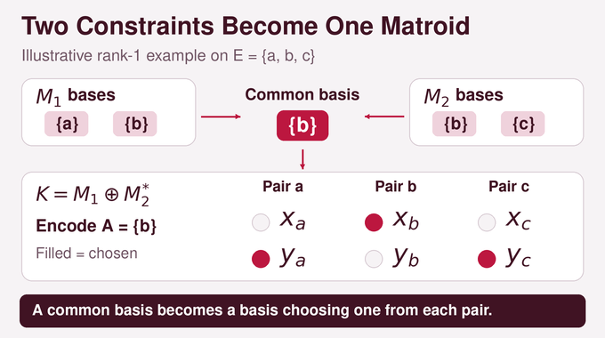
Make two copies of every ground element, called and , and pair corresponding copies. Put the first matroid on the x-copy and the dual of the second on the y-copy:
The dual’s bases are complements of the original bases. Its rank is , so this direct sum has rank . Independence in a direct sum means independence separately in each component.
A transversal chooses exactly one element from every pair. For a subset of the original ground set, choose when and otherwise. The resulting set contains elements. It is a basis of precisely when its two components attain ranks and .
The first requirement makes a basis of . The second makes its complement a dual basis, equivalently making a basis of . This proves an exact bijection between transversal bases and common bases. Transversals themselves include invalid candidates, which becomes useful rather than inconvenient in the weighted construction.
06. Rank-Deficiency Weights and Defect States: Making the Counting Process Work
For an n-element subset of the doubled ground set, rank deficiency measures how far it falls short of full rank. Assign:
The parameter satisfies . Bases have weight one. Other sets have smaller but strictly positive weights as decreases. Write for the transversals and for their total weight, which gradually approaches the desired count.
The chain also admits sets with one empty pair and one full pair, all other pairs singly occupied. Let denote the class with pair empty and pair full, and its unmultiplied weight total. Ordered indices matter because reversing the hole and the full pair changes the class.
A multiplier rescales each defect class. Ideally it equals , making every class’s multiplied total equal the transversal total. The algorithm learns approximate multipliers instead of computing those inaccessible sums directly.
Positive weights guarantee possible paths, but paths can cross states of negligible probability. Balancing defects addresses that bottleneck quantitatively. Connectivity is merely the beginning of the argument.
07. How Lorentzian Polynomials Supply the Critical Inequalities
The algebraic foundation is Brändén and Huh’s homogeneous Tutte polynomial theorem. For the relevant parameter range, it gives a Lorentzian polynomial. The property needed here is concrete: quadratic polynomials obtained by differentiation and nonnegative linear substitutions have Hessians with at most one positive eigenvalue.
A Hessian is the matrix of second derivatives. Its signature limits the directions in which the associated quadratic form is positive. The proof uses this constraint for both selected-element and omitted-element generating polynomials, with duality supplying the second perspective.
After fixing a partial transversal assignment , write for its remaining transversal weight and for its defect totals. Lemma 3.2 gives and, for distinct indices, .
These inequalities prevent incompatible defect totals from all becoming large simultaneously. They guide which pair to condition on and bound the cost of transferring conditional means. The generating polynomials support the proof. The implementation never has to construct their exponentially many coefficients.
08. The Transport Inequality: How Signed Flows Connect Conditional Distributions
Lemma 4.1 compares weighted means in two classes distinguished by which singleton slot is missing. Other slots contain two elements. Allowing a hole in an ordinary slot creates intermediate states connected through one-element exchanges.
The proof constructs a signed current on that exchange graph. Its divergence equals one normalized conditional distribution minus the other. In electrical language, one class supplies current and the other receives it. Signed flows are analytical objects, rather than transition probabilities.
Recursion processes the ordinary slots and distributes demands between their two choices. Each node keeps total weighted demand zero. The omitted-element quadratic form controls the extra energy charged when a slot is split. At the leaves, local clique flows realize the remaining demands.
Conservation then expresses the difference of conditional means as a sum of currents times function differences across edges. Cauchy–Schwarz bounds its square by flow energy multiplied by exchange energy. The resulting coefficient depends on class totals, multipliers, and doubled-slot totals. This is the bridge from polynomial geometry to the random walk’s usable variance bounds.
09. The Metropolis Chain and Observable Poincaré Inequality
The enlarged chain stays put with probability one half. Otherwise it proposes removing a uniformly selected element and adding a uniformly selected outside element. Invalid occupancy patterns are rejected. Valid proposals receive the Metropolis acceptance probability , where includes the defect multiplier.
Its stationary distribution is proportional to those weights. Good multipliers lie within a factor four of their ideal values, ensuring that transversals and each defect type have inverse-polynomial stationary probability.
Define by retaining every value of a function on transversals and replacing values within each defect class by their conditional mean. Proposition 5.3 states:
Here is the chain’s Dirichlet form, measuring weighted squared differences across transitions. The bound preserves all transversal variation and the defect-class means, while leaving arbitrary internal defect fluctuations uncontrolled.
That restriction is deliberate. Type indicators and the counting observables fit this projection. The theorem therefore supplies the statistics needed by the estimator without asserting a polynomial spectral gap for the full chain. Describing it as unrestricted rapid mixing would erase the proof’s central distinction.
10. Trace-Chain Mixing and Warm Starts: Obtaining Reliable Estimates
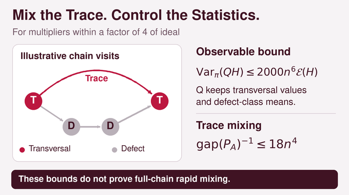
The trace chain records successive visits to transversals, skipping intervening defect excursions. Lemma 6.2 bounds its inverse spectral gap by . Its stationary law is the transversal weight distribution, independent of the multipliers.
The associated mixing estimate also depends on the smallest transversal probability. That probability may be tiny, but its logarithm remains controlled along the chosen schedule. Counting trace steps alone is insufficient, since one step can require several transitions of the underlying chain.
A warm start means pointwise domination by a controlled factor . Lemma 6.1 bounds the mean squared error of correlated time averages of observables fixed by , with dependence on this factor and the observable Poincaré constant. Consecutive samples are not treated as independent.
Adaptive learning makes fresh restarts essential. Once previous observations and endpoints have been revealed, an endpoint need not retain the required conditional warmth. Each phase instead starts from a new uniform transversal and traverses stored annealing levels with independent randomness. Excursion budgets cap actual work, with abort probabilities charged to the error analysis.
11. Annealing and Adaptive Multipliers: Recovering the Common-Basis Count
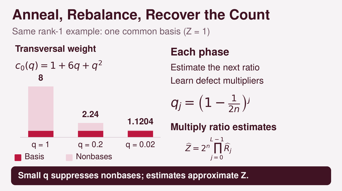
At , all transversals have weight one, so their total is . The schedule uses:
Choose minimally so , and take phases. Between adjacent levels, every state weight changes by a factor between one half and one. Ideal multipliers therefore drift by at most a factor two.
At each phase, empirical type frequencies and the average of estimate the ratio . Updating by multiplying it by restores approximate balance for the next phase.
The final estimator is the telescoping product:
At the last level, bases still contribute exactly one each, while every nonbasis transversal contributes at most . Their combined extra weight is at most . Since feasibility already guarantees a positive integer count, that additive contamination becomes a controlled relative error. Small per-phase estimation tolerances keep multiplication errors within the remaining budget.
12. Why the Algorithm Is Fully Polynomial, and What the Proof Also Establishes
This matroid basis counting algorithm evaluates each state through greedy rank computations using at most original independence queries. Rational weights and multipliers have polynomial bit lengths. Random choices use fair bits with capped rejection trials, and independent bounded runs followed by a median reduce failure to . Unlucky executions cannot run indefinitely.
Corollary 9.1 extends counting to common independent sets of prescribed, unrestricted, or maximum size, even for unequal original ranks. Truncation handles fixed cardinality. Sampling uses successive inclusion and exclusion decisions based on estimated completion counts, with exact feasibility checks keeping every output valid. Almost-uniform means a specified total-variation tolerance, not exact uniformity.
12.1. Evidence and Implementation Limits
| Question | Verified Scope |
|---|---|
| Paper | Explicit oracle algorithm and proofs of approximation and execution bounds. |
| Lean development | Its theorem file records missing concrete bit-operation realization and finite-bit coverage proof. |
| Performance | No application benchmark establishes competitive speed or practical scale. |
The linked Lean theorem file explicitly identifies those model gaps. The formalization repository also asks reviewers to compare definitions with the paper and inspect theorem dependencies. A successful build alone would not settle correspondence. Our Lean proof explainer provides background on that distinction.
The paper leaves its large polynomial bounds unoptimized. Developers should measure oracle costs and estimator variance before expecting useful throughput. As in our Fourier complexity analysis, the computational model determines what an asymptotic claim buys.
Counting Common Bases of Two Matroids offers a precise research target: efficient relative approximation under minimal oracle access. Follow Binary Verse AI’s evidence-focused research coverage, and share a small reproducible implementation that tests these guarantees against exact counts.
What does counting common bases of two matroids mean?
It means determining how many subsets of a shared ground set are bases of both matroids simultaneously. Each subset satisfies both independence constraints and has the common rank. The target is the cardinality of the intersection of their basis families.
Why is counting common bases harder than finding a common basis?
Matroid intersection can find a maximum common independent set in polynomial time, but that does not reveal how many common bases exist. Exact common-basis counting includes bipartite perfect-matching counting, a #P-hard problem. Efficient relative approximation is a separate algorithmic challenge.
What was the main barrier overcome by OpenAI’s proof?
Earlier general oracle algorithms achieved a -factor approximation in polynomial time, while their relative-approximation approach retained exponential dependence on rank . The new paper establishes an FPRAS for arbitrary-rank, equal-rank matroid pairs supplied by exact independence oracles.
Why are Lorentzian polynomials essential to the proof?
Their quadratic signature property yields inequalities controlling defect-class weight totals and the energy of signed transport flows. Those bounds support transversal variance control, the observable Poincaré inequality, and trace-chain mixing used for efficient approximate counting.
Does OpenAI’s proof give an implementable polynomial-time algorithm?
Yes. The paper specifies an oracle-based randomized algorithm with explicit transitions, rational probabilities, bounded random-bit procedures, and polynomial work bounds on every execution. Its estimate has relative error at most with probability at least . An exact pretest detects emptiness and empty inputs always produce zero, although unsuccessful runs on nonempty inputs can also return zero. The paper also derives counting and almost-uniform sampling of common independent sets. The linked Lean development records remaining gaps in concrete bit-operation realization and finite random-bit coverage, and practical competitive performance has not been demonstrated.