
A computer can quickly factor a polynomial by making random choices. Requiring it to make every choice predictably has resisted a comparable guarantee for arbitrary prime fields. OpenAI’s October 4, 2026 manuscript presents a way through that barrier, using geometry to force unknown roots to behave differently.
Deterministic polynomial factorization over prime fields means finding every irreducible factor and its multiplicity without randomness, in time polynomial in the degree and the prime’s binary length. The published manuscript claims exactly that. Its final theorem depends on a separate, unusually strong Hecke zero-free theorem. The result is theoretical, and neither a practical speedup nor end-to-end formal verification is demonstrated here.
Table of Contents
1. What Is Deterministic Polynomial Factorization Over Prime Fields?
The prime field contains residues modulo a prime . Arithmetic wraps around: modulo five, six equals one. A polynomial in has coefficients in this field. An irreducible polynomial cannot be decomposed into lower-degree nonconstant polynomials over the same field.
For example, over with equal to five, . Complete factorization also records repeated factors and the leading coefficient:
Here the left side is the input polynomial, is its nonzero leading coefficient, each is monic and irreducible, and is its positive multiplicity. The input is a dense list of coefficients, including zero coefficients, rather than a compact circuit or sparse expression.
| Feature | Manuscript Scope |
|---|---|
| Input | A binary prime and a nonzero dense polynomial. |
| Output | Leading coefficient, distinct monic irreducible factors, and multiplicities. |
| Size Parameter | , where is degree and . |
| Final Dependency | Companion theorem on finite-order Hecke L-functions. |
| Excluded Resources | Randomness, integer-factorization oracle, primitive-root oracle, and GRH assumption. |
| Evidence Status | Published preprint; no entry found in the current Lean catalogue. |
The encoding matters. A loop through all residues can be exponentially long in . This is the same discipline of specifying the computational model emphasized in our DFT complexity analysis.
2. Why Did Previous Polynomial Factorization Algorithms Need Randomness?
Berlekamp made finite-field factorization a linear-algebra problem. Cantor–Zassenhaus used random choices to obtain expected polynomial running time. Random elements often assign different values to different hidden factors, making them easy to separate.
Deterministic polynomial factorization already had important algorithms. The missing guarantee was uniform polynomial bit complexity in both degree and characteristic length. Shoup’s method has characteristic dependence , which is too large for that goal.
Conditional results require equal care. Under GRH, Rónyai obtained polynomial bounds for a bounded number of irreducible factors. Evdokimov’s general-degree bound is quasipolynomial in degree. Neither statement can simply be relabeled an unconditional uniform polynomial-time solution.
The randomized vs deterministic polynomial factorization distinction concerns how separators are constructed, not whether an answer can be checked. Multiply the returned factors, and you can verify reconstruction. That verification does not tell you how to find them efficiently. Our common-basis counting explainer likewise distinguishes an algorithm’s probability guarantee from its output specification.
3. What Exactly Does OpenAI’s Deterministic Factorization Proof Establish?
Theorem 1.1 claims deterministic polynomial-time factorization with an absolute implied constant and this bit-operation bound:
The exponent is deliberately generous. Its mathematical contribution is being fixed across all input degrees and primes. Polynomial means an asymptotic complexity class, not a promise that anyone should run this bound on a laptop.
Theorem 1.2 isolates the algebraic engine. Set . If and , supply an auxiliary prime for every prime . Its cost is , with the largest supplied prime, or two when none is required, and absolute.
Crucially, this depends on the primes’ numerical values, not just their bit lengths. Polynomially bounded auxiliary primes are therefore essential. In the other branch, enumerating field elements is permitted because the characteristic itself is bounded by a fixed power of the input parameter.
The OpenAI polynomial factorization proof belongs to the October mathematics release. Model provenance supplies context, while the theorem’s correctness rests on its mathematics. Our earlier AI proof coverage explains why those questions need separate assessment.
4. How Berlekamp Algebra Separates Unknown Polynomial Roots
For a square-free polynomial, the quotient algebra represents arithmetic modulo that polynomial. Its Frobenius-fixed elements satisfy . Each unknown irreducible component contributes one prime-field coordinate, so the dimension of this Berlekamp algebra counts the irreducible factors.
The driver constructs a separating element whose multiplication characteristic polynomial is square-free and totally split over the prime field. The geometric splitter then works on this auxiliary polynomial. It does not assume the original input already has only linear factors.
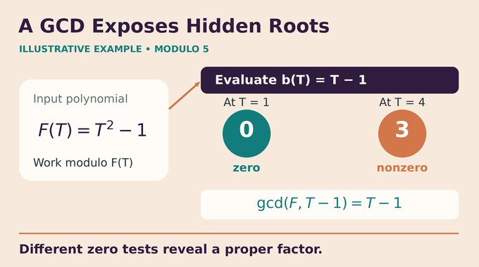
Write for a totally split polynomial whose roots remain unknown. Computing with the residue of the variable performs the same instructions at every root simultaneously. A zero test that succeeds at some roots and fails at others exposes a nontrivial divisor through .
Here is a computed algebra element and is a candidate scalar.
For the earlier quadratic example, testing whether the root equals one isolates the factor with that root. The implementation obtains this through polynomial arithmetic. It never needs a preliminary list of roots. This technique, dynamic evaluation, supplies the proof’s computational interface.
5. Auxiliary Primes and Primary Generators: Replacing Random Choices
For each small prime , an auxiliary rational prime satisfies:
The final condition says the characteristic is not a qth power modulo the auxiliary prime. Taking invariants in a cyclotomic algebra constructs a degree-q field without factoring the large cyclotomic polynomial defining that algebra.
From it, linear equations produce generators of primary multiplicative subgroups, meaning elements whose orders are powers of . For two, the construction produces a quadratic nonresidue and the full two-primary generator. For odd primes, it also constructs the required root of unity.
These generators support promised root extraction through small-prime digit logarithms. This does not require factoring or solving arbitrary discrete logarithms. The related multiplicative-order background appears in our Artin primitive-root explainer.
The small prime fixes the digit alphabet. Even when the subgroup has large order, its logarithm can be recovered one digit at a time by testing a bounded number of possibilities. The algorithm counts those tests and the lengths of the exponents it uses.
There is an apparent circularity: constructing the odd-prime entry requires factoring a cyclotomic polynomial. Its degree is only . Building entries in increasing prime order ensures that this call uses previously constructed entries. The dependency descends strictly in degree, closing the induction rather than introducing an oracle.
6. Even-Degree Factorization: Why a Tournament of Roots Guarantees a Split
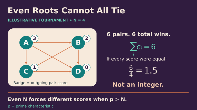
Suppose is totally split, square-free, and has even degree , with odd characteristic and . Consider every pair of distinct roots. The two-primary generator allows the algorithm to label their differences so that reversing the difference reverses the selected orientation.
Think of a tournament: each pair contributes one win to exactly one endpoint. The total scores satisfy:
If all scores were equal, each would be , which is not an integer for even . Consequently, two roots must receive different scores. Since the characteristic exceeds the root count, reducing the scores modulo the characteristic cannot erase that distinction.
A trace computation produces these scores simultaneously, and a GCD selects one score class. With four roots, six matches cannot give all four vertices equal integer scores. With three roots, a directed cycle gives everyone one win. That odd-degree possibility explains why the elegant tournament argument needs a much deeper companion.
7. Odd-Degree Factorization: The Cyclic Curve Behind the Proof
Choose an odd prime dividing the odd root count . Over a carefully constructed finite extension, form the smooth projective curve associated with:
The field contains a primitive root of unity . The curve’s symmetry and its associated operator are:
The points are ramification points, indexed by the unknown roots. There are rational points at infinity. The genus is , so the geometry grows with the input and cannot be treated as fixed.
A divisor is an integer-weighted combination of points. The Jacobian organizes degree-zero divisors modulo principal divisors, those arising from rational functions. It is an abelian variety, with background in our abelian-variety explainer. Here its role is computational.
On the geometric Jacobian, division by is possible. On the lattice of degree-zero divisors supported at infinity, the operator is injective but not universally divisible. Retaining an actual infinity divisor alongside each divisor class preserves this obstruction. Keeping only its class would discard precisely the information needed to force separation.
8. How Norm Equations Make Jacobian Division Computationally Possible
An existence argument alone cannot deliver an algorithm. The deterministic polynomial factorization proof must actually compute the promised divisions without first factoring the unknown point supports.
The manuscript represents finite divisor data with fractional ideals and polynomial matrices. Riemann–Roch reduction replaces divisors with equivalent representatives of controlled size. Large coefficients at infinity are stored in binary, while product circuits represent functions compactly instead of expanding enormous expressions.
A promised Jacobian division reduces to a norm equation in the cyclic function-field extension. The norm multiplies a function’s conjugates under the curve symmetry. Finding a function with the required norm supplies the principal-divisor correction needed for division.
The proposed solver constructs maximal orders in a split cyclic algebra, computes global sections through finite linear systems, and extracts a rank-one idempotent. That matrix-like element determines a norm solution.
An idempotent squares to itself. Rank one means its matrix representation projects onto a one-dimensional subspace, extracting the small piece needed to recover the desired function.
This is specialized machinery with explicit promises and characteristic bounds. The paper checks those conditions in the large-characteristic branch. It does not claim a universal inexpensive norm solver. Uniform bounds on the curve, extension fields, matrices, and function descriptions are all necessary to justify the finite field polynomial factorization algorithm.
9. From Forced Root Separation to Complete Polynomial Factorization
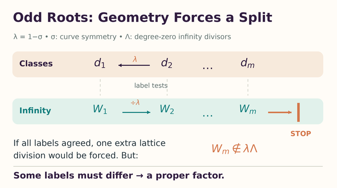
Write , the exponent of dividing , and . The algorithm repeatedly lifts the classes through , sums the lifts, and evaluates labels at ramification points. Subscript zero marks a chosen infinity point.
A Frobenius filtration proves the required divisions are rational over an extension of degree over the root-of-unity field. The total extension degree is at most . Without this control, a finite construction could still require exponentially large representations.
The labels combine two kinds of information: a divisor’s coefficient at each ramification point and the root-of-unity logarithm of a normalized function value there. Their defining function records the difference between applying the symmetry operator to a divisor and subtracting the tracked infinity divisor. Its norm is a constant, and the manuscript proves that the required normalizing root exists in the working field. These are certified promises, not additional guesses.
Let . The infinity lattice has the decisive boundary:
If every reached label test were constant across roots, each would force another lattice division. At the last stage, that would cross the displayed boundary, a contradiction. Therefore some test distinguishes roots and returns a proper factor.
An earlier zero test can also terminate with a factor. If every component keeps agreeing, the geometric contradiction guarantees eventual disagreement. Although intermediate arithmetic uses an extension field, the returned monic divisor selects a subset of roots already in the prime field, so its coefficients belong there too.
The driver transfers that split back through the Berlekamp algebra and recurses. Derivative GCDs handle repeated factors. When the derivative vanishes, the polynomial is a pth power, and recursion multiplies the recovered multiplicities by . Constant inputs return an empty factor list. These steps turn a root-separation theorem into complete factorization.
10. Why the Hecke Zero-Free Theorem Removes the GRH Assumption
The analytic dependency is Theorem 1.2 of the primitive-root companion. It claims that every finite-order Hecke L-function over every cyclotomic field containing the twelfth roots of unity has no zero where:
The principal character is included, with its pole at permitted. There is no conductor or height restriction. Our zero-free-region explainer clarifies why a fixed boundary differs from a corridor that narrows with arithmetic complexity.
The factorization paper uses this input in a smoothed prime-ideal estimate. Comparing a cyclotomic field with a Kummer extension detects primes that fail complete splitting, precisely the auxiliary primes required earlier. Proposition 11.3 bounds them by , with an absolute constant.
Upward search, trial division, and modular exponentiation can then find them within a fixed polynomial budget. Polynomial factorization without GRH therefore relies on the companion’s asserted theorem. The algebraic reduction does not. GRH would independently supply a sufficient zero-free strip for that reduction, but the final claim invokes the companion instead.
11. Is OpenAI’s Deterministic Factorization Proof Practical or Primarily Theoretical?
Primarily theoretical. The manuscript gives no demonstrated advantage over established randomized implementations. Its huge exponent certifies the requested complexity class while leaving optimization and useful runtime unresolved.
For developers, multiplying the outputs verifies reconstruction of the input. Irreducibility requires separate checks. Such tests validate a particular output, while the proof must justify termination and cost for every admissible input.
| Question | Supported Interpretation |
|---|---|
| Deterministic Bit Complexity | Claimed for dense prime-field inputs using the companion theorem. |
| Practical Performance | No demonstrated implementation speedup follows from the bound. |
| Modular Square Roots | Factoring yields roots when they exist. |
| RSA Integer Factorization | No algorithm for factoring an unknown composite modulus is supplied. |
| General Derandomization | A solution to this problem does not establish . |
The RSA distinction is fundamental: the input here already supplies a prime characteristic. Factoring a polynomial in that field differs from finding the prime divisors of a large integer. Likewise, general polynomial identity testing concerns compact arithmetic computations, beyond this dense univariate input. Our Subset Sum analysis illustrates why a problem-specific advance should retain its actual scope.
As checked on October 14, the formalization catalogue contains no matching entry for this manuscript or its primitive-root companion. That is not a disproof. It does mean there is no catalogue evidence for calling their full dependency chain machine-checked. Our Lean verification explainer covers the distinction.
Independent scrutiny should examine the analytic input, promised divisions, and uniform bit accounting. Deterministic polynomial factorization over prime fields would be a substantial derandomization result if the argument holds. Follow Binary Verse AI for source-based analysis of its verification, revisions, and eventual algorithmic consequences.
What is deterministic polynomial factorization over prime fields?
It decomposes a polynomial in into irreducible factors using choices that do not depend on randomness. The manuscript claims a uniform algorithm with running time polynomial in the degree and the binary length of , including factor multiplicities. Its final theorem uses a companion Hecke zero-free theorem.
Why was deterministic polynomial-time factorization difficult?
Randomized algorithms can efficiently choose elements that separate unknown irreducible factors. Earlier deterministic methods did not provide the required unconditional polynomial-bit-time bound uniformly in degree and . The manuscript constructs separators using algebraic and geometric methods, with auxiliary primes supplied by its analytic dependency.
How does the proof factor polynomials without knowing their roots?
It performs computations simultaneously in a quotient algebra representing unknown roots. Whenever a zero test gives different outcomes on different components, a polynomial greatest common divisor can isolate a nontrivial factor. Berlekamp algebra connects this splitting procedure to arbitrary square-free inputs.
Why does the proof treat even- and odd-degree polynomials differently?
For an even number of roots, a pair-orientation argument ensures their integer scores cannot all coincide. With odd degree, equal scores are possible. The manuscript instead uses cyclic curves, Jacobian divisor classes, and an infinity-lattice obstruction to force distinguishable labels.
Does OpenAI’s polynomial factorization proof require the Generalized Riemann Hypothesis?
The stated final theorem does not assume GRH. It relies on a uniform Hecke zero-free theorem from a companion manuscript to guarantee sufficiently small auxiliary primes. The algebraic reduction is established separately from that analytic input, whose correctness is essential to the final unconditional claim.
Does the complexity exponent of 10¹² make the algorithm practical?
No practical efficiency follows from the stated bound. It supplies a theoretical polynomial-time guarantee with an extraordinarily large exponent. The manuscript does not demonstrate that its construction outperforms established randomized algorithms on realistic inputs.
Does deterministic polynomial factorization break RSA or prove P = BPP?
No. Factoring polynomials over differs from factoring large integers, so this result supplies no RSA integer-factorization algorithm. It would imply deterministic modular root extraction for explicitly represented polynomials, but does not establish . General polynomial identity testing remains a separate derandomization problem.