
How many pairs of dots can be exactly one unit apart? Every pair in an equilateral triangle of side one qualifies. Add a fourth dot, and getting all six pairs to qualify is already impossible in the plane. The Unit Distance Problem asks how fast the maximum count grows with the number of points. OpenAI’s September 2026 preprint proves that the count grows at most as a fixed power strictly below , improving the exponent set in 1984. The proof gives no numerical value for the improvement. Its central move is to show that configurations approaching the old exponent would have to satisfy incompatible geometric and algebraic constraints.
Table of Contents
1. What Is the Unit Distance Problem? Start With a Simple Drawing
For a set of distinct points in the Euclidean plane, count each pair at distance one once. Let be the largest such count over all placements of the points. The norm in the formula is ordinary Euclidean distance, and the braces around the two endpoints denote an unordered pair.
The triangle has three unit pairs out of three possible pairs. The square has four out of six because each diagonal has length . Two points one unit apart have just two possible common neighbors at unit distance. Those neighbors are apart, so adding both cannot complete a configuration of four mutually unit-separated points. For another question that starts with the same unit-distance graph, see Binary Verse AI’s coverage of the Hadwiger–Nelson coloring problem.
| Question | Maximum number of unordered unit-distance pairs among points in the plane |
|---|---|
| Classical Bound | Spencer, Szemerédi and Trotter, 1984. Exponent . |
| New Bound | OpenAI, September 2026. A fixed exponent below . |
| Open Quantity | The value of the exponent saving and the exact growth rate |
2. Why the 4/3 Upper Bound Survived for 42 Years
Paul Erdős posed the repeated-distance problem in 1946. Rescaling the plane makes any chosen positive distance equal to one, so the numerical choice of unit does not restrict the question. In 1984, Joel Spencer, Endre Szemerédi and William T. Trotter established the classical upper bound. Draw a unit circle around every point. Each unit pair produces two incidences, one for each choice of center. Two distinct circles meet at most twice, and two distinct points lie together on at most two unit circles.
In a later crossing-number proof, László Székely connected consecutive points along the circles to build a graph. Once the graph has enough edges, the crossing inequality forces crossings to accumulate, while circle intersections limit how many crossings can occur. Balancing those constraints recovers the exponent. For related geometry, see crossing numbers of complete graphs and the Falconer distance problem, which studies distances in a different setting.
Subsequent work improved the leading constant and described structure near the incidence scale. The preprint also cites a logarithmic improvement conditional on a rigidity conjecture. A smaller constant, or even division by a fixed power of a logarithm, leaves the exponent unchanged. The new proof needs further constraints on how incidences fit together.
3. What OpenAI’s Unit Distance Proof Actually Establishes
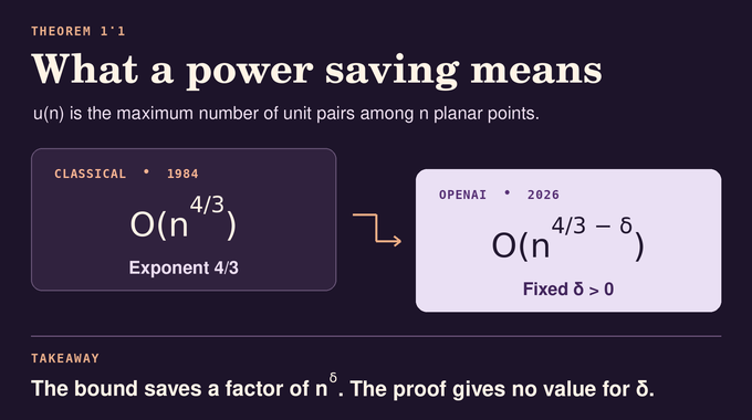
Theorem 1.1 of A Power Saving for Planar Unit Distances gives absolute constants and such that for every nonnegative integer . Equivalently, set to express the improvement as a subtraction from the old exponent.
Relative to the old power, the new bound gains a factor of . For example, multiplying the input size by multiplies that saving factor by . The unspecified prevents a numerical estimate of the gain or a practical crossover point. The proof rules out every sequence approaching the old exponent without supplying a quantitative rate. OpenAI dated the manuscript September 23 and shared the work in its October 6 research release.
4. The Proof Begins by Assuming the 4/3 Exponent Cannot Be Improved
Suppose every fixed improvement fails. For progressively smaller exponent reductions, the proof can choose counterexamples of progressively larger size, because increasing the proposed constant can cover any finite range. Write along this sequence. The ordered count is , where the term denotes an exponent error tending to zero. The use of ordered pairs only doubles the count.
The proof next replaces the original coordinates with real algebraic coordinates. For each configuration it writes down polynomial equations for the required unit pairs, strict inequalities for distinctness, and rational boxes around the original points. The real solution ensures a solution over the real algebraic numbers by the transfer principle for real closed fields. This preserves the required pairs and keeps the new points as close to the originals as desired. The move makes number-field absolute values available later. Our explainer on the existential theory of the reals covers the broader setting of polynomial feasibility.
5. From Unit Circles to an Incidence Graph With Little Shared Information
Make a bipartite graph with a point copy and a center copy of the configuration. An edge means that the point lies on the circle of the given center. Randomly sampled circles partition the plane into cells. The cutting argument and a subsequent restriction extract an unbalanced piece with controlled degrees and an expansion estimate that limits how much edge mass small vertex subsets can capture.
Choose a retained edge uniformly and write for its point marginal. Points therefore carry weight proportional to their degrees. A wedge is sampled by drawing a center according to its edge marginal and then drawing two of its neighbors and independently, with replacement. Each endpoint has law . Their joint law, denoted by , satisfies
Here is relative entropy, the average log likelihood ratio comparing the joint law with independent draws from . Each distinct endpoint pair has at most two possible centers. Controlled degrees limit the weight each center contributes to such a pair, and repeats have vanishing probability. Together with the size of the point side, that bounds the mutual information on the logarithmic scale. For a separate use of mutual information in a proof, see the Courtade–Kumar conjecture.
6. How Short-History Prediction Turns Entropy Into Geometry
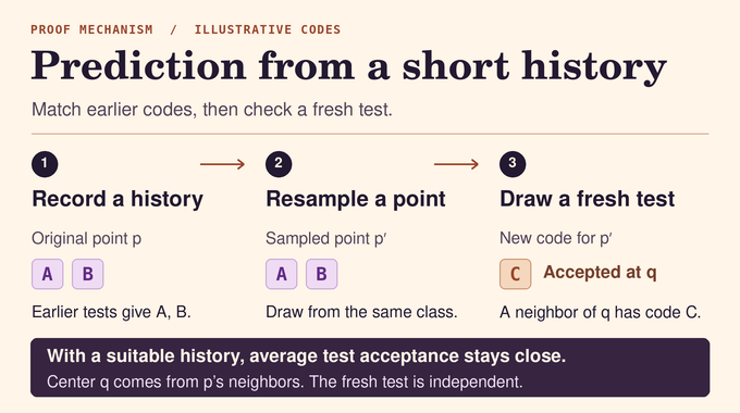
A test gives each point a finite code. A history records its codes on earlier tests. Given an original point, the proof draws a predicted point from the same history class using the point marginal conditioned on that class. If the original point is drawn from the point marginal, averaging over classes gives the prediction that same marginal. The center is sampled from the original point’s neighbors, and a fresh test is drawn independently of the history and the sampled points and center.
The entropy budget limits the cumulative dependence revealed by successive tests. A short enough history keeps the number of classes small, so the predicted point rarely equals the original. A long enough history makes the difference between their average test acceptance probabilities small. The test may use the center to decide which codes qualify. For instance, it can accept a predicted code if any actual neighbor of that center has it.
This is a way to produce a different point with compatible test answers. The prediction need not be adjacent to the center. Keeping the test fresh lets the proof combine acceptance with geometric estimates made under the original marginals. In the bounded case, one prediction can pass the test at three sampled neighbors of the same point.
7. Algebraic Heights and the Bounded-Scale Contradiction
Write and for a point with real coordinates . Multiplying the coordinate differences gives the squared Euclidean distance. For a unit edge between and , this gives
If the first jump is , the second is . Algebraic height measures a number’s size across all normalized absolute values of a number field, including complex embeddings and prime-based absolute values. The product formula makes the weighted logarithms sum to zero, so height can also be read as half the weighted sum of their absolute values.
At each absolute value and threshold, the proof records a bit for whether the negative log size of the first jump exceeds the threshold. The scale integrates the minority frequency of that bit over thresholds and sums over places with their weights. Unanimous thresholds contribute zero.
If stays bounded on a subsequence, normalization and translation give bounded mean heights for coordinates and jumps. At an independently drawn complex embedding, the tests quantize both coordinates into small bins. One predicted point passes at three centers while staying separated from the original in its first coordinate. Its three unit equations hold approximately. Subtracting the original point’s exact equations and then taking differences between centers gives a two-variable linear system. The determinant stays away from zero because the three normalized jumps are separated and bounded with their reciprocals. The system forces the first-coordinate displacement below its required separation. That rules out bounded .
8. Common and Rare Levels: Why Every Remaining Configuration Must Be Structured
It remains to consider . At a level, meaning an absolute value and a threshold, each vertex gets a pair of labels encoding closeness in its two coordinates. Except for bounded integrated error, exactly one label agrees across an edge, and the bit identifies which one. At prime-based absolute values this follows from the reciprocal jumps. At complex embeddings, randomly shifted grids control how often a short jump crosses a cell boundary.
Common levels are those where both bits have appreciable frequency. On most rare levels the minority bit is scarce and one coordinate label dominates. The proof discards rare levels with large consistency error because their total weighted length is negligible relative to . It measures exceptions to the dominant label on the remaining rare levels.
The score estimates reward selected endpoint matches and charge disagreements between edge bits. The product formula bounds their integrals. Prediction and the geometry of pairs of labels supply lower estimates, including a comparison that transfers concentration from history samples to the actual point. Combining point-centered and center-centered scores cancels rare-level terms. Two conclusions survive. Common levels account for negligible center-wedge variation relative to , and rare-level exceptions at points retain positive mass on the scale . That surviving mass drives the extraction.
9. High-Height Ratios and the Rectangle Identity
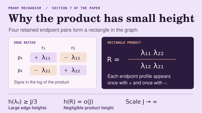
For a pair of wedge endpoints and , choose a surviving witness center . The ratio of their first-coordinate jumps and the alternating product for four retained pairs are
The four ratios can use different centers. Here a rectangle is the set of four graph edges joining two left vertices to two right vertices. At each absolute value, the log size of a retained ratio is approximately a difference of endpoint profiles. Every profile appears twice with opposite signs around the rectangle, so only the errors survive.
The proof removes errors by their height-weighted mass before selecting a common band. Discarding a small fraction of wedges by probability alone could erase a large share of the height. The result is a graph with at least pairs, a scale , individual heights at least , and rectangle products of height uniformly. Pairs sharing any real unit circle that contains at least retained point-side vertices are removed, even if that circle’s center was absent from the incidence graph.
10. The Final Algebraic Obstruction That Forces a Power Saving
Section 8 passes to a field built from sequences of the algebraic data. Elements of negligible height relative to form a relatively algebraically closed subfield. Any ambient element algebraic over this subfield already belongs to it. Each rectangle product belongs to this subfield, while each individual ratio is transcendental over it. Differentiating with respect to a derivation that kills the subfield converts the multiplicative relations into additive constraints on logarithmic derivatives.
The graph contains a fixed complete bipartite pattern whose positions are jointly generic over the coefficients of their plane or curve loci. Genericity here means they satisfy only the polynomial relations imposed by their loci. After adjoining the positions and derivative data on one side, a dimension count ensures that at least one point on the other side remains generic over that enlarged field.
The squared distance between two endpoints can be written in terms of their ratio because their jumps at the witness center are reciprocal in the other coordinate.
Solving for the ratio brings in a square root with radicand , where is that squared distance. The proof finds a valuation for each radicand at which it has odd order and the others have order zero. This makes their square classes independent and permits independent sign changes. The popular-circle deletion removes the common unit-circle case in which this argument can fail.
In the rank-two case, three differentiated equations determine the unknowns using only the first three radicals. Changing the sign of a fourth leaves those unknowns fixed but forces an equality the derivation was chosen to avoid. The same-line case uses two equations and a third sign change. The contradiction eliminates the unbounded-scale branch.
11. What the Proof Verifies and What the Unit Distance Problem Still Leaves Open
The Lean 4 proof module contains the formal upper-bound theorem. The Erdős Problems verification record reports building it and matching it to the pinned comparator statement. Separately, OSVerify’s manuscript review identifies an overgeneralization in Section 8.2. Genericity can fail after adjoining points to an already enlarged coefficient field. The review proposes restricting automatic preservation to the original base field. Section 8.3 establishes the needed genericity over its enlarged field by a separate dimension count. The formal check covers the theorem statement and its Lean proof.
The May 2026 construction cited in the paper disproved Erdős’s proposed near-linear upper bound by producing superlinear powers along an unbounded sequence of sizes. The September paper bounds every configuration from above. On the construction side, Eric Naslund’s October preprint reports a computer-assisted lower exponent of 1.043171 along a sequence of sizes. The exact growth rate of the Unit Distance Problem remains open, and the new upper bound gives neither an explicit exponent nor a recipe for building extremal configurations.
What changed after 42 years is what the geometry permits at large scales. Counting incidences reaches the old exponent. Following the dependencies between those incidences, through prediction and algebraic height, rules out configurations that would approach it. Follow Binary Verse AI for more research explainers on Erdős’s similarity conjecture and Lean formalization of Fermat’s Last Theorem.
1. What is the Erdős unit distance problem?
The unit distance problem asks for the maximum number of unordered pairs of distinct points exactly one unit apart in a set of points in the Euclidean plane. Paul Erdős introduced the problem in 1946.
2. What is a simple example of the unit distance problem?
An equilateral triangle of side length one has three unit-distance pairs. A unit square has four, one per side. Its two diagonals have length .
3. Why was the 4/3 exponent so difficult to improve?
The classical point–circle incidence estimates control how often points lie on unit circles and yield the exponent. A fixed improvement required further restrictions on how those incidences can fit together. The September proof obtains them through information theory and algebraic heights.
4. What does a power saving mean in the unit distance problem?
It replaces with for some fixed positive . The proof establishes that this saving exists and gives no numerical value for it.
5. Did OpenAI completely solve the Erdős unit distance problem?
The exact asymptotic growth rate remains open. OpenAI’s May 2026 construction disproved Erdős’s proposed near-linear upper bound. Its September proof improved the universal upper exponent.
6. How does OpenAI’s proof improve the 42-year-old upper bound?
It assumes that configurations can approach the old exponent and derives a contradiction. The proof combines a point–circle incidence graph, entropy-based prediction, algebraic heights and a final obstruction using quadratic radicals.
7. Has OpenAI’s unit distance proof been verified in Lean?
Yes. OpenAI released a Lean 4 proof of the upper-bound theorem, and the Erdős Problems verification record reports a successful build and a match to the pinned comparator statement. Separately, OSVerify identified a genericity overstatement in the prose manuscript and proposed a repair. The formal check covers the theorem and its Lean proof.