

A gas of radiation can fill anti-de Sitter space at low temperature. Heat the system enough and a large black hole takes over. The Hawking Page transition is that abrupt switch. In 2003, physicists asked whether its gauge-theory counterpart still switches abruptly when the interactions are weak. A November 2026 preprint on the Hawking–Page transition at weak coupling computes the number that decides.
It finds for the leading quartic coefficient of the Polyakov-loop action, with measuring interaction strength. The negative sign means large- super Yang–Mills theory on a three-sphere has a single first-order deconfinement transition at sufficiently weak nonzero coupling. It happens slightly below the Hagedorn temperature. The distinction is between the temperature where confinement stops winning and the temperature where it stops being locally stable.
Table of Contents
01. Hawking–Page Transition at Weak Coupling
| Feature | Result or Scope |
|---|---|
| Theory | super Yang–Mills on a spatial three-sphere |
| Regime | Leading large and weak positive coupling |
| Transition | One first-order jump into a gapped deconfined phase |
| Temperature | Below the Hagedorn limit of metastable confinement |
| Evidence | Three-loop perturbative calculation reported in a preprint |
The two phases are equilibrium states of the same thermal system. The transition is first order because the energy and the magnitude of the Polyakov loop jump when those states exchange dominance. Their free energies are equal at the transition. The discontinuity occurs in the temperature derivative of the free energy, which determines the entropy.
The preprint evaluates the coefficient through the first order at which it can appear, proportional to the square of the coupling. A matrix model translates that sign into a phase diagram near zero coupling. The calculation uses the ordinary thermal partition function of the gauge theory, with all physical states counted by their Boltzmann weights.
02. The Original Hawking–Page Transition and Its Gauge-Theory Dual
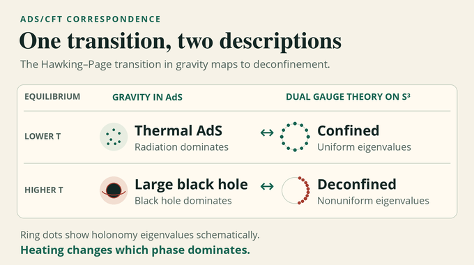
Anti-de Sitter space, or AdS, has a negative cosmological constant. With reflecting boundary conditions, it behaves like a box that lets radiation come to thermal equilibrium. Hawking and Page found in 1983 that the dominant state at low temperature is thermal AdS, a gas of radiation in that box. Above a minimum temperature, two Schwarzschild–AdS black-hole solutions exist at the same temperature. The small one has negative specific heat and is unstable in the fixed-temperature ensemble. The large one is locally stable and eventually has lower free energy than thermal AdS.
In Witten’s 1998 gauge-theory interpretation, the gravitational transition corresponds to a confinement–deconfinement transition on the boundary three-sphere. At large and strong coupling, gravity supplies the calculation. On the gauge-theory side, the thermal free energy changes from order one in the confined phase to order away from coexistence in the deconfined phase. The latter scaling reflects how many adjoint colour degrees of freedom can contribute.
The thermal circle also gives the two descriptions a common diagnostic. It can shrink to a point at a Euclidean black-hole horizon. In thermal AdS the circle cannot shrink to a point. The corresponding gauge-theory observable is the magnitude of the Polyakov loop.
03. The 2003 Problem of One Abrupt Transition or Two Continuous Ones
In their 2003 large-N phase-diagram analysis, Ofer Aharony and four collaborators showed how weak interactions could lift a degeneracy in the free gauge theory. One possibility was a single first-order transition below the Hagedorn temperature. The other started with continuous deconfinement at the Hagedorn temperature. Only on further heating would the eigenvalues of the thermal holonomy stop covering the entire circle. The appearance of that gap would mark a separate third-order transition.
This distinction changes the interpretation of the Hagedorn temperature. With two continuous transitions it would be the equilibrium deconfinement point. With a first-order transition it would lie above the equilibrium switch and mark the end of metastable confinement. The question was therefore whether the weakly coupled system passed through an intermediate deconfined phase with an ungapped eigenvalue distribution, or jumped directly into a gapped phase.
At zero coupling the potential is flat over a range of Polyakov-loop values at the transition temperature. That makes the free result compatible with either outcome as soon as interactions lift the flat direction. Strong-coupling gravity identifies the phase structure at the opposite end of the coupling range. It supplies no value for the coefficient that lifts the degeneracy near zero.
04. From Gauss’s Law to the Hagedorn Temperature
On a compact sphere there is no boundary through which net colour flux can escape. Gauss’s law requires physical states to be gauge singlets. Even when the interaction strength tends to zero, the thermal trace must therefore count singlets. Averaging the trace over the gauge group projects onto those states, much as averaging phases removes components that transform nontrivially. The integration variable is a single unitary matrix , the holonomy around the Euclidean time circle.
At large , the eigenvalues of form a density on that circle. The group measure pushes them apart. The thermal weight from field modes pulls them together, more strongly as the temperature rises. Write for the bosonic and signed fermionic weights of modes winding times around the thermal circle, and for the corresponding Fourier moment. Combining the repulsion and attraction gives the free action
The first coefficient vanishes when the single-letter partition function reaches one. In the paper’s unit-radius convention this happens at
The superscript zero denotes the free theory. Long gauge-invariant single traces can be built by combining elementary field modes, which the paper calls letters. The number of such states grows exponentially with energy, making the confined partition function singular at the free Hagedorn temperature. At that temperature the first Fourier moment can move over a finite interval at zero cost in the leading action.
05. The Polyakov Loop and the Sign of the Quartic Coefficient
The holonomy records how a colour vector changes under parallel transport around the thermal circle. Write for its moments. The first, , is the normalized traced Polyakov loop. Its magnitude is zero for the uniform, confined saddle and nonzero for a deconfined saddle. Averaging over the symmetry-related phases can make the complex loop average vanish even when the saddle has nonzero magnitude.
Near the transition, the first moment is the only one that becomes light, meaning its quadratic cost goes to zero. After eliminating the heavier moments, the action takes the form
Here is the temperature-dependent quadratic coefficient and weights the fourth power of the loop magnitude. In the free theory, if only the first moment is present, the density remains nonnegative exactly for . Beyond one-half the minimum-cost distribution is gapped and further concentration costs extra action. This density constraint supplies the stabilizing rise missing from a negative quartic polynomial on its own.
With , that rise allows a second minimum to form while the origin still has positive curvature. With , the minimum instead moves continuously away from zero once the curvature changes sign. At leading order, reaching one-half then opens the gap and produces the third-order Gross–Witten–Wadia transition.
06. Why the Three-Loop Calculation Took 23 Years
Aharony and collaborators computed the sign in pure Yang–Mills theory on a small sphere in 2005. The supersymmetric theory adds six scalars and four fermion species alongside the gauge field. Their scalar, Yukawa and gauge interactions add many ways for virtual states to contribute. In Coulomb gauge all the species also carry colour charge and enter the instantaneous Coulomb interaction. Individual contributions can diverge, so a consistent way of limiting the high angular momenta and combining terms is part of the calculation.
Planar integrability is powerful for a different job. The leading large- spectrum of single traces determines the growth of states and hence the Hagedorn temperature. Within a single trace the planar dilatation operator can act like a spin chain. The quartic term, by contrast, probes interactions that split and join traces. Those colour contractions cannot be recovered from the planar single-trace spectrum. The full set of two-loop matrix elements needed here had not been supplied by calculations in restricted field sectors.
The distinction is also visible in the same theory’s nine-loop planar scattering-amplitude calculation. A higher loop count in a planar observable gives no access to the trace-changing information that controls this thermal transition.
07. How the Hamiltonian Calculation Works
Radial quantization maps scaling dimensions of local operators to energies on the cylinder with spatial section . The dilatation operator , which measures those dimensions, therefore serves as the Hamiltonian in units of the inverse sphere radius. Its free part counts the energies of the letters. The one- and two-loop corrections shift and mix states. The thermal trace is evaluated with the holonomy insertion so that the powers of stay visible throughout the calculation.
The paper expands the fields in spherical harmonics and fixes Coulomb gauge. The free Hamiltonian is a collection of oscillators, and solving Gauss’s law introduces instantaneous interactions. Many different words of letters have the same free energy. Fourth-order degenerate perturbation theory is needed to construct the effective Hamiltonian within those equal-energy subspaces, with virtual transitions outside them supplying the energy denominators.
In the thermal trace, the squared one-loop insertion and the single two-loop insertion can be separated by their powers of inverse temperature. Of the two-loop operator, the calculation needs a tree kernel that scatters three letters into three and a virtual-loop kernel that scatters two letters with double-trace colour structure. Closing their thermal lines gives the four holonomy traces required for the quartic term. The method targets those contributions directly instead of reconstructing the entire two-loop operator.
08. The Four Contributions That Fix the Three-Loop Sign
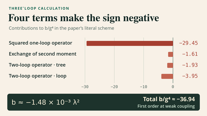
The quartic term receives both a direct four-trace contribution and an indirect one from the second moment. The cubic interaction couples to . The heavier second moment can adjust in response to a nonzero first moment, lowering the action. Eliminating it gives a negative correction proportional to the squared cubic coupling divided by the positive quadratic coefficient of the second moment. The other signs require calculation.
| Source | Contribution to |
|---|---|
| Square of the one-loop operator | −29.45 |
| Exchange of the second moment | −1.61 |
| Tree part of the two-loop operator | −1.93 |
| Loop part of the two-loop operator | −3.95 |
| Total | −36.94 |
The first two entries add to about −31.06 in the paper’s units. Their division depends on how the calculation organizes terms, and their sum is invariant under the scheme change tested in the paper. With and , the total of about −36.94 times gives the leading result
The dimensionless thermal coefficient of the two-loop dilatation operator is about −2.234. It would have to exceed +11.79 to turn the net quartic coefficient positive. This comparison measures how far the computed answer is from a sign reversal. The sign of the two-loop contribution was unconstrained at the outset, which is why it had to be calculated.
09. Three Saddles and a First-Order Transition
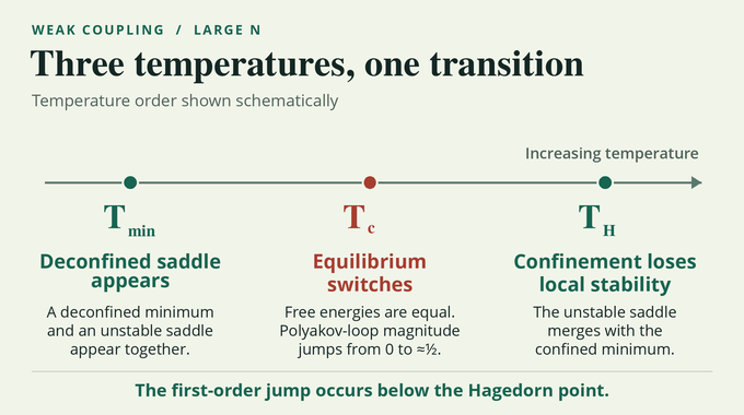
As the temperature rises, falls. To leading order the deconfined minimum and the intervening unstable saddle appear when . To see where the new minimum wins, substitute into the quartic action. Its value relative to the origin is . The actual minimum is just beyond one-half, but to this order the equality of free energies is at . At the crossing the loop magnitude jumps from zero to approximately . The appearance, crossing and loss of confinement define , and , respectively.
From to the deconfined state is metastable, meaning it is a local minimum with higher free energy. From to confinement is metastable. The unstable saddle moves toward the origin and merges with the confined minimum at . These three branches parallel thermal AdS, the large black hole and the unstable small black hole. The loss of local stability of thermal AdS at a Hagedorn point belongs to the string description beyond classical gravity.
The paper’s leading relative separation is . For example, at this gives roughly 3.75 parts per million. The temperature window shrinks quadratically toward zero coupling even though the leading latent heat remains , with the sphere radius.
10. What the Checks Establish and Where Uncertainty Remains
Appendix C describes independently written programs using different representations of the vertices and contractions. A separate vacuum-diagram calculation checks part of the Hamiltonian computation. The loop kernel’s higher series coefficients, starting at the seventh power of the paper’s expansion variable, come from one engine. Those terms contribute about −0.34 to the loop kernel’s −1.50. Restricted sectors provide exact checks on selected matrix elements. In nine near-BPS limits, where only letters saturating a supersymmetry bound survive, the preprint also finds negative quartic coefficients.
For pure Yang–Mills, the paper reproduces the two-loop benchmark to six digits and closely matches six of seven grouped three-loop contributions. The remaining Coulomb and sextic group differs. For a separate comparison, the planar calculation gives −10.71 for a coefficient inferred to be −10.7287 from Harmark and Wilhelm’s two-loop Hagedorn result. That test prompted the discovery of a finite Coulomb counterterm. Its value was fixed against exact operator energies and still lacks an analytic derivation. The Coulomb and mass counterterms lack the four-trace structure needed to shift the quartic coefficient at this order. The candidate double-trace counterterm cancels between bosons and fermions.
The preprint’s provenance statement describes an internal Claude model prompted by a physicist who checked known cases. Anthropic’s release announcement identifies the model as Fable 5.2. The provenance statement also reports a second Claude calculation whose details are outside the preprint. External reproduction of the full coefficient and peer review of the manuscript are separate forms of scrutiny.
11. What the Result Means for AdS/CFT Across Couplings
The Hawking–Page transition is first order in classical gravity at strong coupling and in the gauge calculation at weak coupling and leading large . In both, a stable high-temperature branch and an unstable intermediate branch appear before the stable branch overtakes the low-temperature state. On the weak side, these are saddles of the Polyakov-loop action. A classical spacetime interpretation would require control over the gravity description in that regime.
A continuous first-order line connecting the two regimes is consistent with the result. Establishing it would require following the free energy of the deconfined branch through intermediate coupling. Integrability can track the Hagedorn temperature through the planar spectrum, while determining the equilibrium crossing calls for the free energies of both phases. More immediate tasks include resolving the pure-glue discrepancy, deriving the finite Coulomb correction and checking how chemical potentials change the sign.
The central finding is a separation of two events that coincide in the free theory. Once weak interactions lift the degeneracy, the system changes phase before confinement loses local stability. Follow Binary Verse AI’s coverage of black-hole research and AI-assisted gauge-theory calculations for more on how these results are derived and checked.
1. What is the Hawking–Page transition?
It is a first-order thermodynamic transition between thermal anti-de Sitter space and a large AdS black-hole phase. Through AdS/CFT, it corresponds to confinement–deconfinement in the dual gauge theory.
2. What question about the Hawking–Page transition remained unresolved since 2003?
Whether weakly interacting 𝒩 = 4 super Yang–Mills theory on a three-sphere has a single first-order transition or two successive continuous transitions. In the large-N matrix model, the sign of the quartic Polyakov-loop coefficient selects the outcome.
3. Why does a negative quartic coefficient establish a first-order transition?
The eigenvalue-density constraint stabilizes a separate deconfined minimum while the confined minimum still exists. When their free energies cross, the equilibrium Polyakov-loop magnitude jumps to a nonzero value.
4. Why was the three-loop calculation so difficult?
The gauge field, six scalars and four fermions all contribute, and individual terms can diverge. The calculation also needs trace-splitting and trace-joining interactions outside the planar spectrum used to determine the Hagedorn temperature.
5. Is the Hagedorn temperature the same as the Hawking–Page transition temperature?
At weak nonzero coupling the equilibrium transition occurs slightly below the Hagedorn temperature. The Hagedorn point marks where the already metastable confined phase loses local stability.
6. Has the new three-loop result been independently verified?
The preprint reports independently written implementations within the project and comparisons with known results. A pure Yang–Mills benchmark discrepancy remains, and a finite counterterm used in the Hagedorn check awaits an analytic derivation. The checks reported in the paper do not constitute external reproduction of the full coefficient.
7. Does the result prove the Hawking–Page transition remains first order at every coupling?
The perturbative result establishes first-order behavior at sufficiently weak positive coupling and leading large N. The behavior at intermediate coupling remains open.