

Give a finite automaton permission to walk back and forth across its input, and it can revisit a choice point as often as it likes. Can that freedom make up for losing nondeterminism? OpenAI’s one-way liveness preprint gives a family for which the answer is no. A nondeterministic machine can recognize the language with states and no left moves, while every equivalent two-way deterministic machine needs exponentially many states in , the number of points underlying each relation. The alphabet is finite for each and grows with it. The proof turns repeated head motion into products of matching diagrams, then shows that a small diagram cannot preserve everything those relation products can reveal.
Table of Contents
1. One-Way Liveness and the 1978 Sakoda–Sipser Problem
Sakoda and Sipser asked how many states it takes to replace nondeterminism with a two-way deterministic finite automaton. The machines recognize regular languages, so the issue is how compactly they can describe the same language. A nondeterministic machine accepts when at least one permitted computation succeeds. A deterministic machine follows a single computation from its initial configuration, with one read-only head and one finite control state at each step.
One-way liveness is the witness family that Sakoda and Sipser showed to be complete for the one-way-source version of the conversion problem. OpenAI’s September 25, 2026 preprint uses this family to prove a lower bound even when the target can reverse anywhere on the input. For another example of separating computational models by their resources, see Binary Verse AI’s coverage of time–space tradeoffs for Turing machines.
| Feature | What the Paper Shows |
|---|---|
| Decision problem | Does any path survive the full sequence of relation letters? |
| Nondeterministic source | states, with right moves and stays. |
| Deterministic target | An exponential state lower bound with arbitrary head reversals. |
| Alphabet | All binary relations on points, a finite alphabet that grows with . |
| State measure | Finite control states, including initial and accepting states. |
2. How One-Way Liveness Works With Binary Relations and Surviving Paths
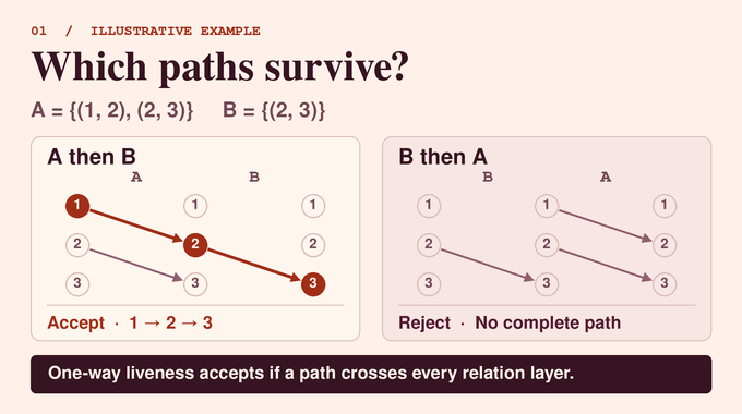
Write for the point set and for its binary relation monoid. Each input letter is one subset of . The product is read in path order. If precedes , a pair belongs to when some intermediate point connects the first step to the second step . The operation is associative. Its identity consists of all self-pairs, and denotes the empty relation.
Here the star denotes all finite words over the relation alphabet, and is the word length. The empty word has product and is accepted. For three points, let contain the pairs 1 to 2 and 2 to 3, and let contain only 2 to 3. Only the route survives both letters, giving . Reversing the letters gives , since the first step ends at point 3 and the next letter has no outgoing pair there. The question is whether a path crosses every layer.
3. Why a One-Way Nondeterministic Automaton Needs Only Three Extra States
The source automaton uses one state for each point and three more for initialization, acceptance, and rejection. On the left endmarker it moves right into any point state. At a relation letter, it can advance right into any point linked from the current one. If there is no such point, that branch enters the rejecting state with a stay move. A branch that reaches the right endmarker in a point state enters the accepting state with a stay move.
In the example above, the branch starting at point 1 advances to 2, then to 3, and accepts at the marker. The branch starting at point 2 advances to 3 on the first letter and then fails. The initial state handles the choice of starting point even for empty input, where the first right move goes directly to the right endmarker. Each branch tracks a single endpoint. A deterministic one-way machine can track the entire set of reachable endpoints, giving a state upper bound of exponential order.
4. The Previous Quadratic Bound and Why It Was Not Enough
Earlier exponential separations constrained the target’s head. In Sipser’s sweeping model, the machine can reverse only at an endmarker. Kapoutsis obtained an exponential separation with sublinearly many reversals as a function of input length. An unrestricted target may reverse at interior cells and make arbitrarily many reversals as inputs grow.
Chrobak had shown a quadratic lower bound for unrestricted deterministic two-way targets using unary languages. In 2026, Kehinde Adeogun and Christos Kapoutsis established an lower bound for unrestricted 2DFAs recognizing one-way liveness. Kapoutsis had also determined the optimal order under the promise of exactly three relation letters. That promise limits word length while keeping the full relation alphabet. The new result applies at every word length. Related Binary Verse AI coverage examines the dependence of Weisfeiler–Leman complexity on the computational task being measured.
5. OpenAI’s Exponential State Lower Bound and the Exact Theorem
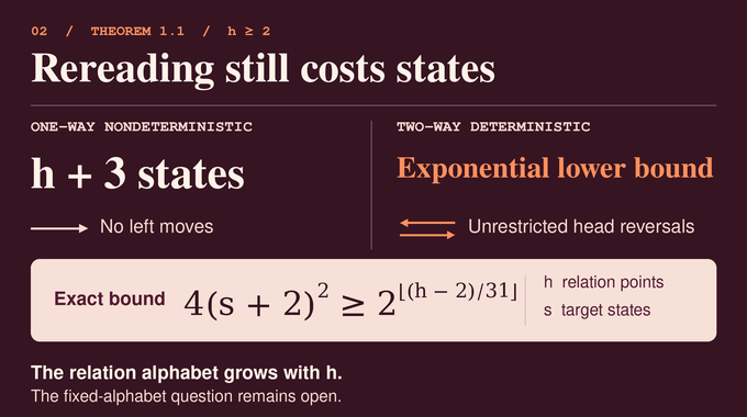
Theorem 1.1 gives a nondeterministic recognizer with states and no left moves for every integer . If an equivalent two-way deterministic automaton has states, the theorem gives the following inequality.
The floor rounds down. Taking a square root and solving for the state count gives the explicit lower bound below.
Because counts states, any fractional lower bound can be rounded up. The estimate is asymptotically , although the explicit inequality can be weak for small . The target has a single head, begins at the left endmarker, and respects both boundaries. Stay moves and partial transition rules are allowed. A computation that runs forever without accepting rejects. When the initial configuration itself can count as accepting, the theorem strengthens the left side to .
6. Why Rereading the Input Cannot Replace Nondeterministic Choices Cheaply
Rereading lets the deterministic head use its position and the symbols it encounters as part of the computation. A proof that simply counts what the machine remembers after a single pass would miss that advantage. OpenAI instead summarizes what a block of input can do when surrounded by other letters. The summary comes from the machine’s configuration graph and accounts for visits from either side.
The language answers one yes-or-no question, but a block’s full relation product can matter later. A context can force the block to start at one particular point and finish at another. If the block summary loses the corresponding entry, the machine cannot distinguish those surrounded inputs. The 1NFA to 2DFA state complexity argument therefore needs a representation that preserves relation products under concatenation.
7. From Two-Way Computations to Trees and Local Matching Diagrams
A configuration consists of a state and a cell position. OpenAI redirects accepting configurations into a new state that moves right to a designated sink at the right endmarker. In the undirected successor graph, the sink component consists exactly of the configurations that reach the sink. Each other vertex in that component has one outgoing successor there, so the connected component has one fewer edge than vertices and is a tree.
A doubled tour traverses each tree edge in both directions. At each vertex, it leaves by the incidence following the one on which it arrived in a fixed cyclic order. The tree produces a single tour. Attach test leaves at the initial configuration and at the sink. In the accepting case, opening the tour at those leaves gives two paths connecting the outer left and right test ports.
For the construction to work letter by letter, the wires at a cell boundary must have the same labels regardless of its neighbors. Reserve a slot for every crossing direction and ordered pair of source and target states. The target end always attaches to its designated state. The source attaches to its own state only for the actual transition and uses a separate fresh leaf otherwise. Stay edges remain within a cell. Two travel lanes per slot give ports on each side for normalized states. Contracting internal paths gives a fixed matching for each symbol, including each endmarker. On rejection the two test leaves lie in separate components, so no wire can connect a left test port to a right one. Cycles elsewhere in the graph cannot change this test.
8. Brauer Diagram Monoids, Rank, Support, and Idempotent Corners
A Brauer diagram monoid consists of perfect matchings on left and right ports. Multiply by gluing equally indexed ports along the shared boundary and pairing the remaining endpoints along the resulting paths. Internal cycles can be discarded. The rank counts pairs crossing from left to right, and multiplication cannot increase it. The support records the indices where a diagram fails to join a left port directly to its corresponding right port.
An idempotent satisfies . The corner uses as its identity. When has rank , deleting its prescribed outer same-side pairs and renumbering the remaining ports gives a rank-preserving embedding into . The renumbering follows the cross pairs of , so they become the identity wires in the smaller diagram. Lemma 2.2 also gives two controls. An idempotent of rank has support at most , and a family with one common support set still has a common set of no larger size after sandwiching and reduction. The latter control keeps the next construction within one port budget.
9. The Key Construction With 32 Conjugates and 256 Relation Additions
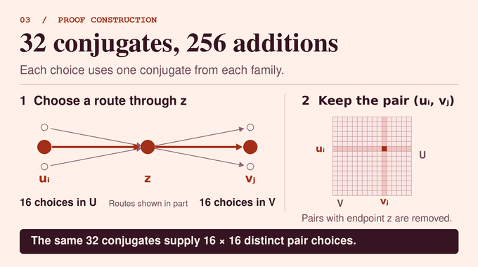
Start with an idempotent diagram that represents the identity relation plus a single off-diagonal pair. Let be its rank loss. Pick disjoint sets and of 16 points each and a separate point . The proof uses permutation-diagram conjugation to produce 16 copies representing an extra edge and 16 representing . These copies all have the same rank as .
Multiplying one copy from each family yields a route from through to . Sandwich the product using a lift of the partial identity on . The outer relations remove pairs with endpoint , leaving that partial identity and one extra pair . The same 32 conjugates supply all 256 pair choices. Since and are disjoint, two added edges cannot compose. Successive additions therefore accumulate by union, with no unintended pairs. The lifted chain uses idempotent powers to preserve those relation images and nest the diagram corners.
10. How the Rank-Loss Induction Produces an Exponential Bound
Let be the decrease in rank at addition , and write for the inductive lower bound on rank loss. All 32 conjugates together touch at most indices, and reduction at the starting partial-identity lift preserves that common support budget. The rank decreases telescope, so this also caps the sum of the losses across the chain.
At each step, retain the two endpoints of the pair about to be added and every point outside . This leaves points. The previous relation restricts to the identity there because the selected pair is still absent. Lemma 2.4 identifies a corner with the full relation monoid on those points. Choosing a minimum-rank idempotent lift gives permutation lifts in the reduced diagram corner. A suitable power of a permutation lift reaches an idempotent over the corner identity. If the lift had already lost rank, that idempotent would contradict the minimum-rank choice. The addition gives one extra pair on the smaller set. Its reduced diagram lift has support at most .
| Quantity | Value and Role |
|---|---|
| Conjugates | 32 diagrams, each supported on at most indices. |
| Successive additions | 256 distinct pairs, one per step. |
| Total rank loss | At most across the entire chain. |
| Points retained per step | , including both endpoints of the new pair. |
| Rank loss per step | At least by induction. |
The induction applies on that smaller set. Summing the 256 step bounds gives the comparison below.
For , the required loss is at least one because an idempotent of full rank is the identity and cannot represent the added pair under a unital map. For , the comparison forces . The resulting lower bound doubles every 31 points.
11. Context Separation Turns Diagram Products Into the Final Lower Bound
Let be the diagram product of the body letters of a word and its relation product. If two words have equal diagram products, the machine gives the same answer in every surrounding context, by associativity and the fixed endmarker diagrams. Suppose their relation products differ at entry . Prepend the singleton identity relation and append . These letters keep precisely that entry when present. Exactly one surrounded word would be accepted, contradicting equality of the diagrams.
Thus the map sending to is well-defined and preserves products and identity. It is onto the full binary relation monoid because every relation is available as one letter. Corollary 3.2 uses a minimum-rank corner to obtain permutation lifts and applies the rank-loss bound there. Its lower bound on the diagram degree , combined with the representation in Theorem 4.1, gives . Proposition 5.1 supplies the small nondeterministic recognizer and completes the separation.
12. What the Proof Establishes, What Lean Checks, and What Remains Open
There are relation letters, since each of the ordered pairs can independently be present or absent. With source states, the lower bound rules out a polynomial state bound uniform over all finite alphabets, even for sources with no left moves. The result leaves the fixed-alphabet determinization question open and measures finite control states. Transition-table size and running time are separate measures.
OpenAI’s math release and the Lean scope notes for family 129 distinguish the liveness theorem from the companion work on complementation. The liveness formalization covers the small source and the deterministic bound under both acceptance conventions, including the sharper bound when an accepting initial configuration counts. The Lean comparator states the target theorem, while the Lean implementation combines the small automaton construction with the deterministic lower bound and formalizes the consequence for polynomial simulation.
One-way liveness gives a concrete reason why revisiting input can leave a deterministic machine exponentially larger. A word that looks like a single yes-or-no test can be surrounded by letters that expose any entry of its relation product, and the machine has to preserve all those distinctions. Follow Binary Verse AI for research explainers on Boolean circuit lower bounds, the Exponential Time Hypothesis, and PCP for PPAD.
What is the one-way liveness problem?
It asks whether the ordered product of binary relations over a finite set is nonempty. Equivalently, does at least one path survive through the entire sequence?
What did OpenAI prove about two-way deterministic automata?
For every h ≥ 2, one-way liveness has an (h + 3)-state nondeterministic automaton with no left moves. Every equivalent s-state two-way deterministic automaton satisfies 4(s + 2)2 ≥ 2⌊(h − 2)/31⌋.
Why can’t a two-way deterministic automaton simply reread its input?
Rereading allows repeated inspection of the input with a read-only head. OpenAI’s proof shows that even unrestricted revisiting requires exponentially many states for this language family.
How does the new proof improve earlier lower bounds?
It strengthens the previous quadratic lower bound for unrestricted two-way deterministic automata recognizing one-way liveness to an exponential one. The proof uses matching diagrams, a common support bound, and inductive rank loss.
Does the proof completely settle the Sakoda–Sipser problem?
It rules out an alphabet-independent polynomial state bound even for one-way nondeterministic sources. The construction uses growing finite alphabets and leaves the fixed-alphabet question open.
Is the exponential lower bound formally verified in Lean?
Yes. OpenAI publishes a Lean formalization of the main theorem under both acceptance conventions. OAI/Combinatorics/Automata/Main.lean assembles the proof, and the comparator file gives the target statement separately.