
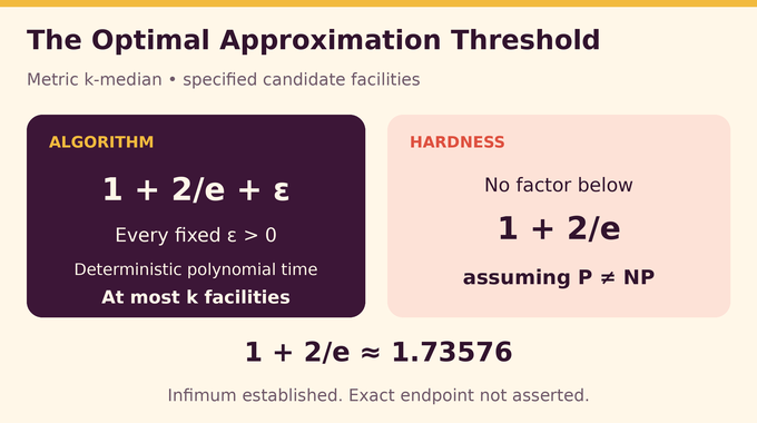
Choosing warehouse locations sounds like a logistics exercise. Requiring a provably near-best choice for every possible metric turns it into a decades-long mathematical challenge. The k median problem asks for at most facilities minimizing total client distance. OpenAI’s September 24, 2026 manuscript presents a deterministic polynomial-time approximation within of optimum for every fixed positive .
That is approximately . Combined with known hardness under , it identifies the optimal approximation threshold for specified candidate facilities. It does not prove that , attain the endpoint without slack, or demonstrate a production speedup. The advance comes from preserving useful information while fractional facilities disappear.
Table of Contents
1. What Is the K Median Problem? The Mathematical Definition
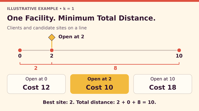
Let denote clients, candidate facilities, and a common metric: nonnegative, symmetric distances satisfying the triangle inequality. Choose a nonempty subset of candidates, with at most members. Each client connects to its nearest selected facility.
For a worked example, put clients at positions 0, 2, and 10 on a line, allow facilities at those positions, and set . Opening at 2 costs , compared with 12 at 0 and 18 at 10. These are ordinary distances, unlike the squared distances in common k-means clustering.
| Research Model | Finite rational metric. Clients and candidate facilities specified separately. |
|---|---|
| Output Budget | A nonempty candidate subset with at most facilities. |
| Approximation | , for every fixed . |
| Running Time | Polynomial in binary input length. The polynomial may depend on . |
| Optimality Condition | Assuming , no deterministic polynomial-time factor below exists in this model. |
The distinction between clients and candidates models a real restriction: demand points need not be legal opening sites. A clinic can serve a neighborhood without being allowed to occupy every patient’s address. The theorem keeps those candidate restrictions explicit.
2. Why Is the K-Median Problem NP-Hard?
Exact optimization requires the cheapest feasible set, not merely a good one. The number of candidate subsets grows rapidly, and the general metric problem is NP-hard. Polynomial time means a running-time bound polynomial in the input’s encoded length, rather than an unrestricted search through all combinations.
An approximation ratio measures the permitted cost relative to the unknown optimum. A factor of 2 allows twice the optimum cost on the worst input. A smaller factor strengthens that guarantee. It does not predict the average gap on a company’s delivery data.
This is why an approximation theorem can advance an NP-hard problem without making exact optimization easy. Our subset sum analysis illustrates another distinction: improving an exponential algorithm also leaves the polynomial-time question unresolved. Here, the improvement concerns the quality achievable within polynomial time.
Worst-case hardness also leaves room for easy individual instances. A line, a small candidate set, or additional geometric restrictions may permit better algorithms. The threshold concerns the unrestricted metric model, so it should not be exported automatically to every clustering variant.
3. The Previous Barrier: From 3 + ε to 2 + ε
Early constant-factor results established that metric structure could tame the search. Bounded-swap local search reached . Later methods combined fractional solutions and bi-point rounding, which interpolates between solutions opening different numbers of facilities.
Li and Svensson made a constant number of extra facilities a useful intermediate allowance. Subsequent rounding refinements reduced the approximation factor. The manuscript’s historical account identifies the following milestones.
| Arya And Coauthors | through bounded-swap local search. |
|---|---|
| Byrka And Coauthors | Corrected guarantee using bi-point rounding. |
| Gowda And Coauthors | 2.613 in the SODA 2023 version. |
| Cohen-Addad And Coauthors | , first announced in 2025. |
| This Manuscript | , with a new directed cost comparison. |
A subsequent graph-based iterative framework also reached . OpenAI builds on that framework, but its general transfer theorem does not supply the smaller factor. As with the factor-2 superstring result, the decisive contribution is proving a stronger accounting bound for a particular construction.
4. What Exactly Does the OpenAI Proof Establish?
Theorem 1.1 of The Approximation Threshold for Metric k-Median states that, for every fixed positive accuracy slack, a deterministic algorithm returns a feasible candidate subset satisfying:
Distances are rational numbers encoded in binary. The input may have arbitrary and separate client and facility sets. The approximation algorithm itself does not assume any separation between complexity classes.
Fixing the slack matters. The theorem allows its polynomial and constants to depend on that choice. It does not promise a uniformly efficient implementation as the requested slack shrinks. Our edit distance approximation explainer discusses a similar need to read fixed-accuracy guarantees carefully.
For intuition, if optimum cost were 1,000 and the slack were 0.01, the bound would be roughly 1,745.76. That is a worst-case ceiling, not an experimental measurement or a statement that every output approaches it.
Binary encoding prevents a hidden numerical shortcut. A distance with many digits contributes those digits to input length. The running-time claim therefore accounts for numerical precision, rather than treating arbitrarily large rational arithmetic as one free operation.
A sensible implementation study would first verify that its distances form a metric and its constraints match this model. Facility capacities, mandatory service levels, and opening charges would require additional analysis. A theorem about total connection distance does not automatically cover those objectives.
5. Why 1 + 2/e Is Optimal if P ≠ NP
The lower bound comes from Max-k-Coverage. Represent each set by a facility and each universe element by a separate client. Incident facility-client pairs have distance 1, nonincident pairs distance 3, and distinct points within either part distance 2.
These distances satisfy the triangle inequality. For example, a same-part distance 2 cannot exceed a two-edge path of minimum length 2. A cross-part distance 3 cannot exceed a cross-part plus same-part path of minimum length 3.
If the universe has elements and the selected sets cover , the connection cost is:
A perfect cover costs . In the hard alternative, at most a fraction is covered, giving cost at least . The known coverage gap under therefore excludes every fixed factor below the threshold.
Together, upper and lower bounds identify an infimum: factors can approach the boundary from above. This differs from a probabilistic transition such as the random 3-SAT threshold. It also leaves the complexity-class assumption intact.
To exclude a proposed factor strictly below the threshold, choose the coverage-gap slack small enough that the induced cost gap remains above that factor. No fixed positive gap excludes the endpoint itself. This is why the strict inequalities in the hardness statement matter.
The constant is Euler’s number, approximately 2.71828. Its appearance is inherited from the coverage gap on the hardness side and recovered independently by the rounding potential on the algorithmic side.
6. The Linear Programming Foundation: Fractional Facilities And Client Assignments
The algorithm begins with a relaxation. Instead of demanding yes-or-no openings, let represent how much facility opens, and let represent client ’s assignment to it.
Every integral solution is feasible for this linear program, so its optimum lower-bounds . Fractional openings provide a cheap starting point, but they are not usable warehouse decisions. Rounding must recover whole facilities without multiplying connection costs excessively.
There is no capacity shared between clients here. Many clients can use the same fractional opening. Splitting a facility into co-located pieces makes assignments easier to track, and merging pieces afterward cannot increase connection cost or facility count. The metric framework also appears in the randomized k-server problem, although that problem concerns online movement rather than static placement.
7. Preparing The Proof: Grid Rounding, Representatives And Supplier Bundles
Arbitrarily tiny opening fractions complicate later updates. Section 3 replaces them with multiples of , where the even denominator depends on accuracy, not instance size. Total opening mass increases by at most , while expected assignment costs suffer an arbitrarily small multiplicative loss.
Separated representative clients define disjoint bundles of nearby mass. A bundle need not contain a full unit. Its deficit records the missing portion, and supplier stars connect that shortage to facilities or other bundles holding usable assignment mass.
The coupling is essential: rounding a shortage separately from its supplier could save nominal openings while stranding clients. One supplier may support many assignments because this is an uncapacitated problem. Signed accounting controls the net mass change, while clipping unusually large deficits protects bundle feasibility.
This produces a carefully structured fractional instance. It has not yet solved the original budget problem. The temporary allowance remains a fixed additive surplus, which later stages must remove.
The preparation proof controls both expected deficits and their variance. Outcomes that exceed the reserved budget are rejected, and the connection-cost analysis includes the conditioning loss. This accounting prevents a superficially cheap fractional construction from relying on unusually expensive budget failures.
8. Tapered Iterative Rounding: How Opening One Facility Erases Others
Each positive grid opening becomes copies of mass . A directed graph tells the procedure which target copies disappear when a source facility opens. Every target chooses exactly incoming source copies, supplying one unit of possible erasers.
Source selection depends on distance through a taper: nearby sources receive stronger inclusion probabilities, with clipping enforcing valid probabilities. The taper relates an erased assignment’s replacement distance to the geometry used in the cost analysis.
Opening and erasure change facility mass in opposite directions. Balanced updates cancel their count effects. Biased unbalanced updates and forced openings for sources with large erasure sets control the remaining imbalance. Opened integral groups persist through resets.
The local operations require global justification, much as switch-chain mixing requires more than plausible individual swaps. Here the critical obligations are connection cost and facility count. The paper bounds them separately before combining their success conditions.
After the rounding rounds, a deterministic completion supplies remaining connections. Its geometric bound also provides the persistent fallback used by the potential analysis. Thus the analysis can track a guaranteed eventual connection even before a currently open facility realizes that bound.
9. The New Argument: Directed Comparison Inequality And Surviving-Assignment Potential
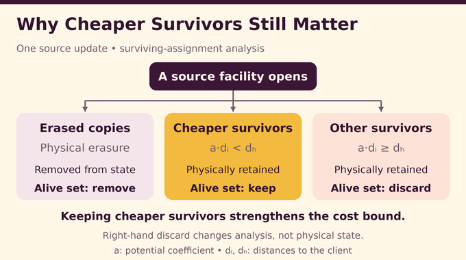
The new analysis refuses to forget every alternative when one assigned facility opens. For each client, it tracks surviving original copies, their total mass , their remaining weighted distance , and a persistent upper bound on eventual connection distance.
At elapsed time , put . The potential is:
Here . The coefficient is its tangent-line value at the surviving mass. Initially , so the potential equals . That identity explains where the final constant enters the upper-bound analysis.
When an original copy opens, cheaper surviving alternatives remain in the analytical alive set. More precisely, surviving copies whose coefficient-weighted distance is below the newly opened distance retain value. This creates a negative correction that can pay for harmful erasures elsewhere.
Theorem 4.1 packages that payment into a finite directed comparison inequality. Normalized distances have weighted mean one, and directed coefficients need not be symmetric. Rows with positive contributions transfer charges toward smaller-distance rows, whose negative contributions cover those charges. Appendix A supplies explicit rational polynomial certificates for the scalar estimates.
Forced openings depend on the realized graph. Their potential change is bounded graph by graph before averaging. Reversing that order would risk unjustified conditioning. This is a specialized proof improvement, not a universal lower-bound technique like those studied in permanent versus determinant complexity.
The potential is not asserted to decrease on every trajectory. The comparison controls averaged drift, while discretization and termination introduce errors absorbed into the accuracy slack. Retaining cheaper survivors supplies the savings needed for that stronger average guarantee.
Evaluating the defining integral at one gives . The rest of the analysis shows that subsequent rounding spends only the allowed additional slack beyond this starting value, rather than repeatedly paying a fresh worst-case replacement bound.
10. How The Proof Becomes Deterministic Without Losing Its Guarantee
A randomized existence argument would be insufficient for the announced deterministic theorem. Section 6 replaces local randomness with rational distributions having polynomial support. It preserves the particular low-order moments used by the analysis, rather than every possible dependency.
Affine support reduction retains feature expectations using at most one more state than the feature dimension. Required features include pair moments and, for a quadratic count statistic’s variance, moments through degree four. The method does not claim arbitrary adaptive behavior survives compression.
Instead, the construction retains physical histories across a constant number of rounds. Each history has polynomially many children, so the full tree remains polynomial for fixed accuracy. Budget failures are discarded, and the cheapest remaining total-cost outcome is selected.
The proof also bounds rational encoding lengths. Small support alone would not control arithmetic costs. This echoes the binary-input issue in mean-payoff games and the separate determinism question in polynomial factorization over prime fields.
Selection uses the sum of client costs. It does not require one outcome to satisfy every client’s expectation bound simultaneously. Moreover, the transcendental clock functions belong to the analysis. The implemented physical choices use rational data and fixed rational approximations.
11. Removing Extra Facilities: How The Algorithm Returns To Exactly k
The intermediate deterministic algorithm opens at most facilities, where depends only on accuracy. Its cost is compared with the assignment LP. This is a constant-additive pseudo-approximation, not yet an ordinary feasible answer.
The established Li–Svensson reduction removes the surplus with an arbitrarily small additional approximation loss. For fixed surplus and loss, its overhead is polynomial. OpenAI first establishes determinism, then applies the reduction. It does not use budget repair to turn an expectation into a deterministic theorem.
The final algorithm opens at most original candidates. If exactly are required, add unused candidates. Distances to the nearest facility cannot increase. Crucially, the argument does not establish the same ratio for rounding the original LP directly to the exact budget.
12. What The Lean Formalization Establishes And What Remains Outside The Proof
The formalization scope notes cover the deterministic approximation and conditional infimum statements. The actual approximation implementation and threshold proof are separate from comparator statements, whose placeholders specify the targets. The comparator instructions describe the verification workflow. We inspected these sources but did not rerun Lean or the comparator.
Formal checking concerns encoded statements and their dependencies. Correspondence with the paper still deserves examination. The hardness conclusion uses specified candidates: requiring changes the lower-bound question. Neither the exact endpoint nor practical efficiency follows from the theorem. As our three-machine scheduling analysis emphasizes, polynomial time can hide enormous constants or exponents.
OpenAI’s mathematics release invites community scrutiny. Publication and formal artifacts support examination, rather than replacing independent validation. For the k median problem, the durable lesson is how surviving assignments sharpen rounding while budget repair preserves feasibility. Follow Binary Verse AI for evidence-led explanations that connect each theorem to its mechanism, assumptions, and limits.
What is the k-median problem?
It selects at most facilities to minimize the total distance from clients to their nearest selected facility. In metric k-median, distances satisfy the triangle inequality. Unlike the common k-means objective, it does not minimize squared distances.
Why is the metric k-median problem NP-hard?
Finding an exact optimal solution is NP-hard in general. The new paper addresses a different question: how closely a polynomial-time algorithm can approximate that optimum while respecting the facility budget.
Did OpenAI prove that P ≠ NP?
No. The approximation upper bound is unconditional. The matching hardness lower bound assumes . The paper does not prove or disprove that assumption.
What approximation ratio does the OpenAI proof achieve?
For every fixed , Theorem 1.1 guarantees a deterministic polynomial-time approximation, approximately , while opening at most specified candidate facilities.
Why is 1 + 2/e called the optimal threshold if the algorithm still needs ε?
Every fixed factor above is achievable. Assuming , no deterministic polynomial-time factor below it is achievable in the specified-candidate model. The threshold is therefore an infimum; attaining the exact endpoint is not established.
How does the new algorithm overcome the previous 2 + ε barrier?
It combines tapered iterative rounding with a directed comparison inequality and a potential that retains cheaper surviving assignments. These strengthen the connection-cost analysis. A deterministic implementation and an additive-to-ordinary reduction then recover a solution within the original facility budget.
Has the k-median proof been formalized in Lean?
OpenAI publishes Lean proof implementations for the deterministic approximation and the conditional threshold, with comparator configurations specifying their target statements. These are meaningful formal artifacts. Correspondence with the mathematical paper and independent verification still matter. We inspected the sources but did not rerun Lean or the comparator.