
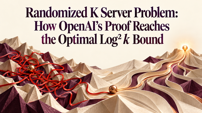
Two mobile servers can spend forever chasing nearby requests while a better plan moves once and stops. The randomized k server problem asks how much that lack of foresight must cost. OpenAI’s September 24, 2026 preprint gives a squared-logarithmic answer: on every metric space, a randomized online policy can stay within a universal constant times of the offline optimum, plus a fixed additive term.
The result matches the known worst-case lower bound. It does not restore the original logarithmic conjecture, which was disproved. Its contribution is a matching upper bound, assembled from changing metric partitions, posterior distributions, fractional allocation, and carefully charged rounding. The proof also covers infinite and unbounded spaces. Understanding how those pieces avoid an extra logarithm explains the advance.
Table of Contents
1. What Is the Randomized K-Server Problem?
Place servers in a metric space: a collection of points with distances satisfying symmetry, positivity, and the triangle inequality. Requests arrive individually. Each names a point that must receive a server. The cost is total distance traveled, not elapsed time, processor work, or prediction error.
For two servers initially at positions 0 and 10 on a line, a request at 4 can be served by moving either server. Moving the left one costs 4. That looks sensible until later requests expose what coverage was sacrificed. “Online” means the decision uses only requests already revealed. Randomization permits probabilistic choices without granting future knowledge.
| Source | OpenAI preprint dated September 24, 2026. |
|---|---|
| Theorem domain | servers, at least metric points, arbitrary initial positions. |
| Guarantee | Expected movement at most times OPT, up to a universal factor and fixed additive constant. |
| Adversary | Oblivious: requests are independent of the policy’s random choices. |
| Scope | Finite, infinite, bounded, and unbounded metric spaces. |
| Important limit | The main paper establishes policy existence without computational-efficiency guarantees. |
2. Competitive Ratio: Why the Nearest Server Can Be Wrong
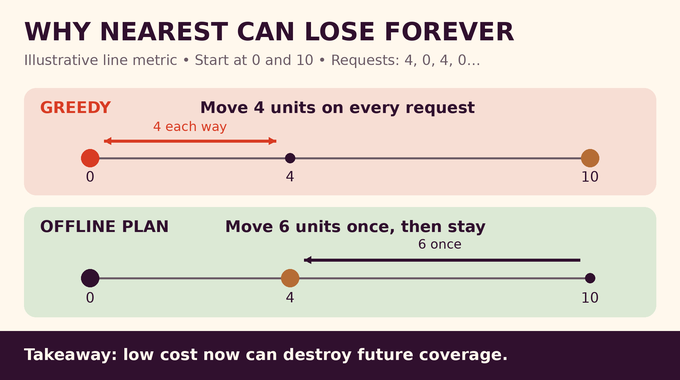
Consider servers at 0 and 10, followed by requests alternating between 4 and 0. Greedy moves the left server from 0 to 4, then back, repeatedly paying 4. The right server remains unused. An offline plan moves the right server from 10 to 4 once, paying 6, while retaining coverage at 0. As the sequence grows, greedy’s ratio becomes unbounded.
Write for the request sequence and for the cheapest legal service when every request is known beforehand. A competitive ratio compares an online policy against that same starting configuration, allowing a fixed additive allowance. The expectation averages the policy’s randomness on each fixed input, not a friendly distribution of workloads.
This is different from the approximation ratio in our shortest common superstring explainer: there the complete input is available. Here the information arrives too late to undo earlier decisions.
3. The Randomized K-Server Conjecture and the Log² k Lower Bound
Paging encouraged the original randomized k server conjecture: perhaps every metric admits competitiveness. In a uniform metric, every move between distinct points has the same cost, and the optimal randomized paging ratio is the harmonic number, which grows logarithmically.
But Bubeck, Coester, and Rabani’s lower-bound construction produces certain -point metrics requiring competitiveness. The conjecture’s universal logarithmic promise therefore fails. The squared-logarithmic obstruction is existential: some metrics require it. It does not say every metric does.
That quantifier matters. Our quadratic sensitivity analysis likewise separates a counterexample from a universal theorem. Here the new upper bound closes the worst-case asymptotic gap, while easier metric families can still admit better ratios.
4. The Previous Barrier: Why Tree Algorithms Were Not Enough
Hierarchically separated trees, or HSTs, organize distances into clusters at geometrically shrinking scales. Their nested structure makes allocation easier. The multiscale entropic regularization paper achieved competitiveness on HSTs. However, transferring through a static randomized embedding of an -point metric adds expected distortion . The resulting general-metric guarantee retains an unwanted dependence on the number of points.
Evolving partitions offer another route: change the representation as relevant mass moves. But changing a representation itself costs money in the analysis. OpenAI’s paper explicitly notes that Lee’s earlier general competitive-ratio claim was withdrawn following a gap. The new argument credits heavy-ball protection as an antecedent while proving its own partition-edit and anchor-travel estimates. It does not assume the withdrawn conclusion.
5. OpenAI Proof: The Optimal Squared-Logarithmic Theorem
Theorem 1.1 of the research manuscript states that, for every integer , every metric with at least points, and every initial server tuple, there exist a randomized online policy and finite such that every finite request sequence satisfies:
Here is universal, independent of the metric and . The additive may depend on the metric, server count, and initial configuration, but never on the request sequence or its length. With distinct starting positions, is possible. One policy works across all sequences and horizons for the specified metric and start.
“Optimal randomized k server” therefore describes asymptotic worst-case order, not an exact leading constant or a measured speedup. The theorem assumes oblivious requests. It supplies no equivalent guarantee against an adversary watching and reacting to random decisions.
6. The Hidden Offline Optimum and Posterior Movement
The proof first fixes a finite metric and a known probability law on finite request sequences. For each possible input, select an offline-optimal trajectory. Its realized future remains hidden. The online construction sees only conditional distributions of that trajectory, updated from the revealed prefix.
A posterior might say that a particular subtree contains two comparator servers with some probability and three otherwise. That information describes uncertainty under the known input law. It does not disclose which future sequence actually occurs. Later minimax and compactness steps eliminate dependence on this preliminary law.
The distinction between filtering and drift carries the accounting. Filtering revises beliefs about yesterday’s hidden configuration after today’s request becomes known. Drift then moves that hidden configuration forward through the comparator’s actual service step. A posterior can change sharply because information arrived, even if little physical movement occurred.
For affine potentials with old coefficients fixed, filtering has zero conditional expected change. For concave potentials it has nonpositive expected change. Drift is charged through a coupling of the old and new hidden states. Crucially, these signed estimates are applied before selecting resets or edits. Selecting only inconvenient updates afterward would invalidate the expectation argument.
For example, observing a request can change the inferred probability that a server occupied a region yesterday. That update is filtering. Moving the designated hidden server from its old point to the newly requested point is drift. The latter has an actual distance budget. Keeping the two operations separate prevents a change of belief from masquerading as physical work.
Thus posterior volatility is not automatically counted as transportation. This separation lets the proof use information about the optimum without paying repeatedly for merely learning where its servers probably were.
7. Evolving Partitions: Heavy Balls and the Logarithmic Telescope
At each geometric scale, the construction builds partitions using the comparator’s posterior counting measure. Its total mass is , since it counts servers rather than normalizing them into a single unit. Heavy balls protect requests near concentrated mass. Other requests use chronological rosters, grouped into doubling qualification tiers.
These rosters track candidate covering balls. Random retirements keep their simultaneous sizes bounded, while a separate short-lived auxiliary roster pays retirement errors. The label alphabet can therefore be fixed independently of the request horizon. A point’s full string of scale labels becomes a leaf of one fixed prefix tree, even though the current metric partitions evolve.
The difficult payment comes from a finite-dimensional variational potential. It minimizes an integral over separated auxiliary sites subject to capacity constraints. Those sites are analytic devices, not extra servers. Concentration forces substantial site weight near a request. Relocating such a site gives local inequalities that pay partition edits.
Why does this cost only one logarithm? The estimates depend on ratios of posterior mass in nearby balls. Across geometrically related scales, the denominator at one scale is controlled by a numerator farther down the chain. Taking logarithms turns products of ratios into sums whose interior terms cancel.
The relevant ratios are local rather than one global measure of the metric’s complexity. A large space may have many points and many distance scales, yet only limited server mass to redistribute. That is why a telescope over masses can replace a charge based on the ambient point count. The proof must also pay for uncovered requests and roster edits, not merely for idealized well-covered locations.
The remaining endpoint mass ranges between a fixed positive floor and order . Consequently the total is . Charging a full logarithm independently at every level would reintroduce metric-size or scale dependence. The telescope avoids precisely that mistake.
8. Tree Allocation: Convex Rank Functions and Parked Server Mass
On the resulting tree, the next task is allocating fractional server amounts. For a vertex , let be its hidden comparator occupancy. Rank probabilities record the chances that this integer count falls below each threshold. Convex, nonincreasing functions of those probabilities produce compatible lower bounds for subtree allocation.
The amounts must cover the requested leaf with at least one unit, keep root mass exactly , and stay bounded by a universal multiple of posterior expected occupancy. Child amounts may sum to less than their parent amount. The difference is parked at the internal vertex instead of being forced into children prematurely.
That parking freedom prevents unnecessary movement when child proportions fluctuate. The proof’s slow-proportions trackers select removals from child allowances while respecting changing constraints. Coarse parameter changes and fine allocation caps have separate budgets, so a logarithmic potential slope does not multiply every adjustment indiscriminately.
A nearly dominant child needs special treatment. The construction assigns the side children first, then gives the dominant child the remaining parent amount, subject to its cap. This preserves compatible bounds without introducing another logarithmic loss. The allocation theorem ultimately bounds weighted fractional tree variation by one logarithm times the embedded comparator’s movement.
Fractional mass is an intermediate mathematical object. A developer cannot implement the result by placing half a physical server at two endpoints. The next step must recover exactly integral servers while preserving both coverage and movement accounting.
9. Balanced Rounding: Turning Fractional Mass Into Real Servers
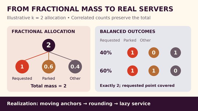
Parked mass needs a representative point, called an anchor, in the original metric. Here a subtle expense appears: the anchor can move while its tree vertex and parked amount remain unchanged. Counting only mass crossing tree edges would miss that travel.
The paper controls retained-anchor motion with an affine potential and a pointwise bound on parked-mass coefficients. This uses the domination of allocated mass by posterior expected occupancy. It pays for moving representatives without multiplying the entire tree-variation budget by another logarithm.
Balanced rounding then converts fractional allocations into integer counts, including parking as an extra child target. Parent and child rounding states may be correlated. Independence would be an unjustified shortcut because their totals must fit together and the requested leaf must remain covered. The rounding lemma incurs only an absolute movement factor.
Finally, a lazy simulation translates these configurations into legal service: do nothing if the request is already covered, otherwise move one actual server to it. A minimum-matching potential pays the discrepancy between actual and simulated configurations. This matching is a transportation comparison, distinct from the graph optimization problem in our maximum cardinality matching analysis.
10. Why the OpenAI Proof Has Exactly Two Logarithmic Factors
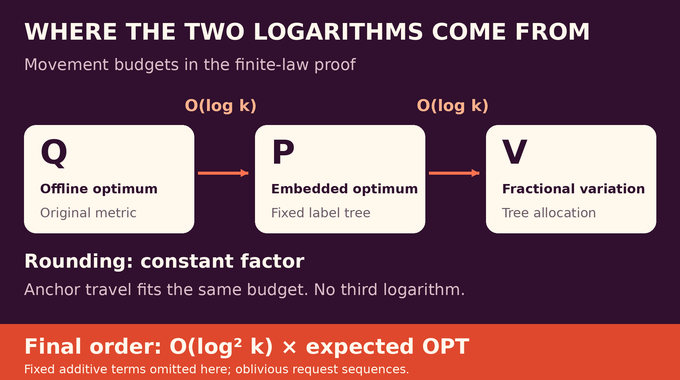
Let be expected offline-optimal movement, embedded comparator movement, and weighted fractional tree variation. Write . Sections 2–9 establish the following accounting, with absolute multiplicative constants:
The additive terms depend on the fixed finite instance and structures, never on the input law, horizon, or number of updates. The first inequality contributes the partition logarithm. The second contributes the allocation logarithm. Their composition gives the square.
This third inequality is decisive. Substituting and leaves every term at most squared-logarithmic in , plus a fixed additive allowance. The anchor contribution already includes , so it fits the same budget. Balanced rounding adds a constant factor, not a third logarithm.
| Partitions | One logarithm: original comparator movement to tree comparator movement. |
|---|---|
| Allocation | One logarithm: tree comparator movement to fractional variation. |
| Anchors and rounding | Preserve the squared-logarithmic order, with fixed additive terms. |
| Lazy simulation | No multiplicative increase beyond the simulated movement budget. |
As in our counting perfect matchings explainer, controlling the transfer between intermediate representations is part of the theorem, not a cleanup detail.
11. One Policy for Every Metric: Compactness, Guarantees, and Limits
This is a k server competitive ratio statement about cumulative movement. It provides no per-request promise that each move is short, and expectation does not become a high-probability guarantee without additional analysis. Those distinctions matter when translating a theorem about adversarial sequences into requirements for a real service system.
The finite-law construction is not yet the final policy. For distinct starts, episode amplification with forward inputs, reversed optimal moves, and reset blocks removes the additive allowance. Finite separation then provides one policy satisfying any finite collection of input constraints. Each request history requires only a probability vector over possible server labels.
Those vectors form a product of compact simplices. Each fixed finite input imposes a closed expected-cost constraint involving finitely many coordinates. Because every finite collection is feasible, compactness supplies a policy satisfying all of them. Unbounded spaces cause no infinite cost on an individual finite input: only finitely many finite distances enter. Repeated starts are handled by comparison with a distinct auxiliary configuration, producing the permitted fixed additive term.
The Lean scope documentation covers this theorem and a separate uniform randomized algorithm for finite rational metrics. That companion gives polynomial preprocessing and per-request time in encoded instance length and request-counter bit length. Its additive movement constant need not be polynomially bounded. Neither statement supplies production benchmarks, a caching deployment, or an adaptive-adversary guarantee.
For developers, movement competitiveness and runtime remain separate resources, as our time-space tradeoff explainer emphasizes. For AI readers, OpenAI’s mathematics release supplies provenance, while formalization and independent expert review answer different questions.
The randomized k server problem now has a matching worst-case asymptotic upper bound in this research package. Its most useful lesson is how geometry, uncertainty, and realization costs are controlled together. Follow Binary Verse AI for research explainers that distinguish theorem scope from verification evidence and trace what an AI-generated proof actually establishes.
What did OpenAI prove about the randomized k-server problem?
The proof establishes an competitive ratio, written precisely using , for randomized online k-server on arbitrary metric spaces against oblivious finite request sequences. It matches the known worst-case lower bound in asymptotic order, with a universal multiplicative constant and a fixed additive allowance that can be zero for distinct starting positions.
Wasn’t the randomized k-server conjecture already disproved?
Yes. The original conjecture predicted competitiveness on every metric. Earlier research established an lower bound for certain metrics. OpenAI’s proof supplies the matching upper bound for arbitrary metrics. It does not say that every metric requires the larger ratio.
Is this the same as the deterministic k-server conjecture?
No. The deterministic conjecture concerns a -competitive algorithm without randomized decisions. This paper establishes a randomized squared-logarithmic guarantee against oblivious requests. These are different mathematical statements and adversary models.
Why does OpenAI’s proof use hierarchical trees?
Trees organize distances and server allocations across scales. The proof adapts metric partitions to local posterior mass, then allocates fractional servers on a fixed tree of label strings. Separate estimates control partition changes, allocation, and moving representatives so that the final multiplicative bound depends only on the server count.
Does the proof work against adaptive adversaries?
The stated theorem applies to oblivious requests, chosen independently of the policy’s random decisions. It does not establish the same competitive ratio against an adversary that adapts requests to those decisions.
Does the result work for infinite metric spaces and practical algorithms?
The existence theorem includes infinite and unbounded metric spaces, without claiming computational efficiency. A separate companion result provides a uniform randomized algorithm for finite rational metrics with polynomial preprocessing and per-request time in encoded input length and request-counter bit length. Its instance-dependent additive movement constant is not claimed to be polynomially bounded. These results do not demonstrate practical deployment performance.
Has the OpenAI k-server proof been formally verified?
OpenAI’s Lean documentation states that the formalization proves the competitive-ratio theorem and the separate uniform-computation result. Machine checking concerns the encoded statements and their derivations. It does not independently referee every explanation in the manuscript or establish practical performance.