
A square looked like a plausible ceiling. OpenAI’s September 25, 2026 paper constructs Boolean functions that break it: for every positive constant , some total function satisfies . That disproves the quadratic sensitivity conjecture, while leaving Hao Huang’s 2019 polynomial Sensitivity Conjecture theorem intact.
The construction combines separated Hamming balls, labelled tournaments, and recursive target-and-gate clauses. Its achievement is controlling how many individual bits can change the output while allowing many disjoint groups to do so. The OpenAI quadratic sensitivity conjecture proof is therefore a separation theorem about Boolean functions, not evidence of faster software or more robust neural networks. Here is where the extra growth comes from.
Table of Contents
1. What Did the Quadratic Sensitivity Conjecture Proof Disprove?
Theorem 1.1 of the original research paper rules out one constant working for every total Boolean function. “Total” means every binary input has a defined output, without a promise excluding inconvenient cases.
Quadratic Sensitivity Conjecture: Key Facts
| Question | Verified Answer |
|---|---|
| What fails? | A universal bound , for any fixed positive . |
| What survives? | The polynomial relationship, including . |
| What is constructed? | Finite, nonconstant total Boolean functions with unbounded . |
| What is not established? | The optimal exponent or an application performance improvement. |
Quantifiers matter: a different function may defeat each proposed constant. One counterexample to coefficient one would not settle that stronger statement. This distinction between improving a bound and settling its parent problem also guides our permanent versus determinant analysis.
2. Sensitivity vs Block Sensitivity: One Bit or a Disjoint Group?
Let , and let mean input with precisely the coordinates in set flipped. For a singleton, write , with an input position. Boolean function sensitivity at an input counts the individually decisive positions:
Block sensitivity is the largest number of pairwise disjoint, nonempty sets whose separate flips change the output. Global and are the respective maxima over all inputs.
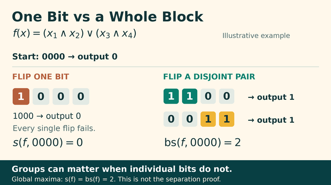
Consider . At 0000, one changed bit cannot complete either AND. Two disjoint pairs can.
A Four-Bit Worked Example
| Change From 0000 | Output and Meaning |
|---|---|
| Flip any one position | Output remains 0, so . |
| Flip positions {1,2}, or separately {3,4} | Each produces output 1, so . |
| Check global maxima | . This illustrates the definitions, not a superquadratic separation. |
Local insensitivity need not mean global simplicity. Nor does it measure information preserved under random noise, the different question in our Courtade–Kumar explainer. Here the comparison concerns worst-case counts of decisive changes.
For the four-bit example, any rejecting input can have at most one almost-complete pair in each AND, giving at most two sensitive bits. At an accepting input, only a single completed pair can be vulnerable, again giving at most two.
At a rejecting input, a successful block must complete a pair by flipping its missing bits. Each pair supports at most one such block in a disjoint family. At an accepting input, every successful block must break an already completed pair. That pair has only two positions to share among disjoint blocks. Thus global block sensitivity also never exceeds two. This checks the global numbers rather than inferring them from zero.
3. The Original Quadratic Barrier and Earlier Constructions
Nisan and Szegedy explicitly suggested the square bound. Rubinstein showed quadratic separation was possible. Virza improved the examples to , followed by Ambainis and Sun’s .
These constructions made the ratio approach a constant. They excluded subquadratic universal bounds but left room for a sufficiently generous quadratic coefficient.
Huang’s 2019 proof settled the polynomial question. His degree bound, combined with Tal’s degree–block-sensitivity comparison, yields . Wellens subsequently improved the leading constant. The new paper attacks the remaining square barrier from below, without contradicting those upper bounds.
For readers following our quantum query complexity coverage, the familiar lesson is to specify the measure and exponent. A separation between mathematical resources does not automatically translate into elapsed-time performance.
4. Why Spectral Sensitivity Was Not Enough
Draw a graph whose vertices are binary inputs. Connect adjacent inputs when changing their one differing bit changes the function. Its maximum degree is . Spectral sensitivity is the operator norm of this graph’s adjacency matrix, with .
Meiburg’s earlier construction used tournament rows, positive conditions, and selected blocking coordinates. The paper adapts that architecture, explicitly acknowledging the source. But a large ratio does not imply a large ratio with : replacing the denominator by a larger quantity can erase the advantage.
The missing ingredient is a direct ordinary-sensitivity bound at every recursive level. As with the resource assumptions in our quantum circuit lower bounds article, changing the measured object changes what the theorem establishes.
5. The Starting Construction: Nested Hamming Balls
Choose depth , integer size parameter , and . Partition bits into disjoint blocks of size . Centre has ones exactly in block , so distinct centres are distance apart.
Hamming distance counts differing positions. With the distance to the nearest centre, define the initial predicates:
Picture concentric shells around isolated islands. Increasing shrinks each accepting ball, giving nested predicates. Adjacent inputs change by at most one, so one bit cannot cross two distinct integer-radius thresholds simultaneously.
A rejecting input within one step of acceptance can approach only one centre. Otherwise two centres would be at distance at most , contradicting their separation. This controls initial rejecting-side sensitivity and makes both initial joint-sensitivity counts zero. Nesting concerns predicate indices, not monotonicity in input bits.
At zero, flipping one whole block lands exactly on its centre and makes every initial predicate accept. These blocks are mutually disjoint. Thus the same starting gadget provides both ingredients needed later: many coordinated ways to cross the boundary and tightly limited ways for one bit to cross it. Neither property alone would establish the final theorem.
6. Labelled Tournaments Prevent a Dangerous Pattern
At each recursive level, arrange disjoint child inputs into rows, each with positions. A tournament assigns exactly one direction to each pair of rows. Choose it so every row has outgoing edges.
Label edge by a position in destination row . The required labelling forbids 16 rows for which every internal incoming edge to each row selects one common position in that row.
Independent uniform labels establish existence. For 16 chosen rows there are 120 edges. Specifying one position per row gives at most choices, each succeeding with probability . The union bound is:
Therefore some labelling avoids every forbidden pattern. This is a finite existence argument, not a measured success rate or an efficient label-search guarantee. The number 16 provides a convenient fixed bound.
7. Recursive Clauses Combine Targets and Rejecting Gates
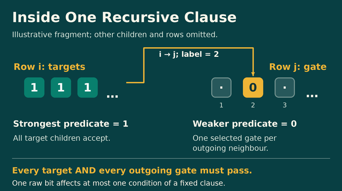
At level , there are predicates. Write , the strongest child index. Clause for parent index requires:
Read this spatially: light every target in row , then require darkness at one selected gate in each outgoing neighbour. The parent accepts if any clause succeeds.
Targets use the strongest predicate. Gates demand rejection of a weaker one. Increasing lowers the gate index, making rejection harder and preserving nesting. Within a fixed clause, every condition uses a different child. Thus one raw-bit flip can affect only one condition of that clause, even though it may affect several clauses.
A predicate here is simply a yes-or-no test on a child input. Each child is itself a complete lower-level construction, rather than one bit. The recursion therefore has two scales: the clause sees child answers, while sensitivity always counts flips of original input coordinates. Confusing these scales would hide precisely the amplification that the proof must control.
8. Why Only a Few Clauses Can Be Repaired by One Bit
Fix a rejecting parent input before choosing a bit. Let contain clauses failing exactly one target and no gates. Let contain clauses failing exactly one gate and no targets. Any clause made true by one flip must belong to these fixed lists.
For row in , call its failed target position . If and , clause ’s passing gate selects a child whose weaker predicate rejects. Nesting forces its strongest predicate to reject too. It must therefore select , row ’s only failed target. Sixteen candidates would create the forbidden label pattern. Hence .
Inside , every row has all targets true. An internal outgoing edge consequently points to a true gate predicate, making that gate fail. Each clause has just one failed gate, so the induced tournament has outdegree at most one. Counting edges gives:
At most one vertex in this induced tournament has outdegree zero. Every other candidate repairs a gate in another fully accepting target row. That repair must flip both the weaker gate predicate and the strongest predicate from one to zero.
The possible exceptional gate lacks this strongest-predicate guarantee. It requires an ordinary-sensitivity allowance. For two parent predicates becoming true together, however, even that gate must cross two distinct child thresholds. Keeping that exception straight is essential to the next estimate.
The lists must be fixed before the flip. Choosing a fresh candidate family after seeing each changed bit would not bound their combined contribution. A coordinate may repair several clauses, but summing their possible repair counts is still a valid upper bound. Overcounting helps here. Omitting a class of possible repairs would invalidate the sensitivity estimate.
9. The Four Sensitivity Recurrences
Define as maximum sensitivity over level- predicates and inputs with output . Define as the maximum count of bits simultaneously flipping two distinct predicates from to , at the same input. Empty maxima are zero. Let primes denote the previous level.
For an accepting input, fix a satisfied witness clause. Any output-changing bit must break a target or gate, explaining the first line. To destroy two accepting predicates through a gate, the bit must change both corresponding child predicates, giving the second.
For rejecting inputs, the candidate counts supply 16 target allowances and three joint gate allowances. Only ordinary rejection sensitivity needs the extra exceptional term. Tracking joint changes prevents that cost from spreading unchecked through recursion.
Normalize by : let and be the maxima over of normalized and , respectively. With , the recurrences imply:
The scaling reflects an imbalance between the two output sides. The accepting-side recurrence has a factor multiplying the previous rejecting-side profile, while the rejecting side inherits one previous accepting-side profile. Giving accepting profiles one extra power of makes both dominant transfers have coefficient one. The remaining coefficients become small or depend on the joint profiles.
Initially and . Choosing makes . A simultaneous comparison induction bounds and through depth . Consequently:
Large suppresses the small forcing of joint sensitivity before its factor-three amplification becomes dangerous. This is the paper’s decisive control of ordinary sensitivity.
To see the induction’s budget, each normalized joint profile starts at zero and receives only a small forcing proportional to . Its accumulated upper bound is a geometric sum in three. Summing those joint contributions back into the ordinary profile costs less than its original allowance , because was chosen exponentially small in the prescribed depth. The bound covers every input, not merely the zero input used for block witnesses.
10. The Quantitative Proof Breaks Every Square Bound
Each level- predicate has disjoint sensitive blocks at zero, each of size . To lift a block, copy it into every child of one target row. All targets switch on together. Other rows stay zero, so all outgoing gates remain satisfied.
Finally OR together disjoint copies of . At a zero input, sensitivities add across copies. At a one input, only a unique accepting copy can contribute sensitive bits. If two copies accept, changing one bit cannot turn the OR off.
Sensitivity Growth Versus Block Growth
| Quantity | Final Bound |
|---|---|
| Ordinary sensitivity | . |
| Block sensitivity at zero | . |
| Input dimension | . Finite, but extremely large. |
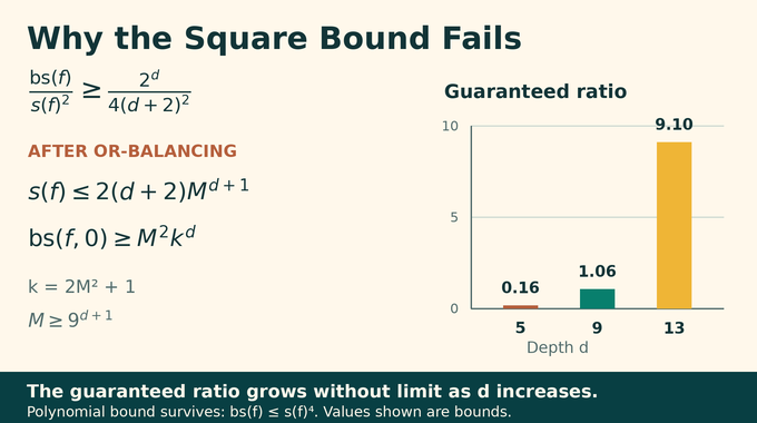
Dividing the block lower bound by the squared sensitivity upper bound gives:
Exponential growth in beats the quadratic denominator. Choose depth to exceed the proposed constant, then choose sufficiently large . That order proves the unbounded ratio. Unlike the algorithmic guarantees discussed in our edit distance approximation article, this construction establishes an obstruction rather than a practical implementation.
The input-size cost is substantial: both the branching factor and the required parameter grow rapidly. The proof needs finite witnesses, not economical ones. Its probabilistic label choice and generous constants are sufficient for disproving a universal inequality, but do not identify the smallest counterexample or the most efficient construction.
11. From One Counterexample to an Exponent Above Two
Depth gives a seed with bounds and , where . Compose disjoint copies repeatedly. Sensitivity is submultiplicative, while zero-input block sensitivity is supermultiplicative when the inner function maps zero to zero.
In disjoint composition, an outer sensitive coordinate is replaced by an entire inner function on fresh bits. A raw bit matters only if it changes that inner answer and the corresponding outer coordinate matters. For blocks at zero, combine each sensitive outer block with each sensitive inner block. The resulting Cartesian-product blocks remain disjoint, providing the product lower bound. Equality is unnecessary for either estimate.
Thus and . Setting yields , with block sensitivity tending to infinity. The optimal exponent remains undetermined between this lower bound and the quartic upper bound.
OpenAI’s Lean formalization notes cover the quantitative ratio, its unboundedness, and the fixed-power result. The proof implementation contains those theorems. The comparator statement is not the implementation. This review inspected sources, not an independent Lean build or completed peer-review record, a distinction developed in our Lean verification explainer.
For researchers, the reusable idea is to control simultaneous threshold changes alongside ordinary sensitivity. For developers, no runtime or robustness benchmark follows. The quadratic sensitivity conjecture falls because recursive blocks outgrow carefully restrained single-bit effects. Follow Binary Verse AI’s AI mathematical proofs coverage for explanations that trace the theorem, its mechanism, and what remains open.
Did OpenAI disprove the Sensitivity Conjecture?
No. Hao Huang proved the original polynomial Sensitivity Conjecture in 2019. OpenAI’s 2026 paper disproves its stronger quadratic version: no universal bound can hold for every total Boolean function with one fixed positive constant .
What is the difference between sensitivity and block sensitivity?
At a given input, sensitivity counts individual bits whose separate flips change a Boolean function’s output. Block sensitivity counts pairwise disjoint, nonempty groups of bits whose separate simultaneous flips change the output. Global sensitivity and block sensitivity maximize these counts over all inputs. The new construction makes block sensitivity exceed every constant multiple of sensitivity squared.
Why did earlier examples fail to disprove the quadratic conjecture?
Earlier constructions achieved separations proportional to sensitivity squared. They excluded subquadratic universal bounds but left open a quadratic bound with a sufficiently large constant. OpenAI’s construction makes unbounded.
How does the labelled tournament make OpenAI’s proof work?
The tournament organizes recursive predicates into directed rows, with edge labels selecting gate positions. Its forbidden label pattern limits target-repair candidates to fewer than 16. Tournament structure limits gate-repair candidates to three. Combined with bounds on simultaneous predicate changes, these constraints control ordinary sensitivity through recursion.
What exponent does OpenAI’s superquadratic proof establish?
The paper establishes a fixed and a family of total Boolean functions satisfying , with zero-input block sensitivity tending to infinity. It does not determine the optimal exponent. The quartic universal upper bound leaves a gap between the demonstrated lower-bound exponent and four.
Has OpenAI’s quadratic sensitivity proof been verified in Lean?
OpenAI publishes Lean 4 scope notes and proof implementations for the quantitative separation, unbounded quadratic ratio, and fixed-exponent result. The linked comparator statement should be distinguished from the proof implementation. This article inspected the published sources but did not independently rebuild the Lean development. Formalization also differs from independent peer review and does not establish an optimal exponent.