

A polynomial can have only two choices for each coefficient and still face an entire circle of tests. OpenAI’s October 5, 2026 manuscript presents a proof that littlewood polynomials with coefficients ±1 can have magnitude arbitrarily close to their natural square-root scale at every angle, for every sufficiently large integer length. The achievement asserted is simultaneous control of peaks and dips, including the easily overlooked real points of the circle.
The mechanism combines oscillatory waves, Fourier analysis, and discrepancy rounding. Its central improvement preserves amplitude while suppressing unwanted endpoint contributions. This is an existence theorem, not a demonstrated fast generator of useful sequences. Also, the linked Lean documentation covers weaker statements than the manuscript’s full two-sided theorem. Understanding both boundaries is essential to understanding the result.
Table of Contents
1. What Are Littlewood Polynomials, And Why Are ±1 Coefficients So Restrictive?
A length- Littlewood polynomial contains exactly consecutive coefficients, each either positive or negative one:
Here is a complex input, labels a coefficient, and selects its sign. Length differs from degree: this polynomial has degree . For example, has length four. At its value is two. At it is negative two. Those checks look promising, but they say nothing about the remaining angles.
Complex coefficients of modulus one can point in any direction. Real Littlewood polynomials permit only two opposite directions. Every sign change alters interference around the whole circle. A local repair can create a distant problem, which explains why searching over sign strings is an awkward substitute for proof.
| Component | Meaning And Scope |
|---|---|
| Source | OpenAI manuscript dated October 5, 2026. |
| Coefficient restriction | Exactly +1 or −1 at all N consecutive positions. |
| Domain | Every point on the complex unit circle. |
| Main statement | Arbitrarily small relative error around the square-root scale at every sufficiently large length. |
| Verification boundary | The linked Lean notes describe weaker results, not the full uniform two-sided theorem. |
2. The Original Erdős–Littlewood Flatness Problem: Why Is The Square Root Of N The Target?
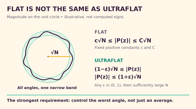
Write , where is an angle in radians. The unit circle consists of all complex numbers with modulus one. Powers of rotate at different speeds, and the polynomial adds these rotating contributions.
Orthogonality makes different frequencies cancel when their products are averaged. Parseval’s identity therefore gives:
The average squared magnitude is fixed regardless of the signs. Consequently, the maximum magnitude cannot fall below . If the magnitude were almost constant, that constant would necessarily be close to . The target is dictated by energy accounting, not aesthetic preference.
The original flatness question asks for positive constant lower and upper multiples of this scale everywhere. Ultraflat polynomials demand much more: the relative error must become arbitrarily small uniformly. Perfect constancy is impossible for a nonconstant Littlewood polynomial, since the highest nonzero Fourier coefficient of its squared magnitude contains the nonzero product of its first and last coefficients. The theorem approaches perfection asymptotically.
3. Previous Barriers: From Rudin–Shapiro To The Missing Lower Bound
Rudin–Shapiro polynomials provide real-sign constructions with maximum at most at power-of-two lengths. That controls large peaks, but does not itself supply the near-optimal positive minimum needed here. Kahane established ultraflatness with complex unimodular coefficients, where continuously adjustable phases provide additional freedom.
The 2020 theorem of Balister and colleagues established two-sided constant-factor flatness for every degree at least two. It answered the classical existence question, while leaving the stronger ultraflat target unresolved. Its degree-based normalization should not be silently confused with the present manuscript’s length convention.
The supplied paper identifies a September 23, 2026 predecessor establishing asymptotically minimal maxima through all lengths. An October 5 refinement additionally obtained a lower bound of . That is meaningful nonvanishing, but a normalized floor of one-sixteenth remains far from one, even when the ceiling approaches one.
There is a useful connection with our Barker sequence explainer: binary signs and cancellation matter in both settings. The constraints differ, however. Ultraflatness does not assert the individual correlation bounds defining a Barker sequence.
4. OpenAI’s Ultraflatness Theorem: Near-Perfect Bounds At Every Angle
Theorem 1 of the Ultraflat real Littlewood polynomials manuscript states that for every tolerance , there is a threshold such that every integer admits signs satisfying:
The same polynomial satisfies both inequalities everywhere, including and . There are no omitted arcs and no restriction to a subsequence of convenient lengths. Nevertheless, the signs may change completely when the length changes.
For a one-percent tolerance, the conclusion means a magnitude between 0.99 and 1.01 times the square-root scale, once the unspecified threshold is reached. This illustrates the quantifiers, not a computed threshold.
The linked Lean scope notes document an asymptotically optimal maximum and convergence in every fixed finite power mean. They do not document this stronger uniform two-sided conclusion. Average convergence can tolerate narrow exceptional dips, whereas uniform convergence cannot. No independent Lean build or peer-review certification is established by this article.
5. The Proof Strategy: Building An Almost-Flat Function Before Choosing Signs
Choosing signs comes last. First, the proof constructs a continuous complex-valued function on the circle with magnitude close to one everywhere. Its retained Fourier coefficients are real and bounded by slightly more than . The absolute sum of coefficients outside the permitted frequency range is negligible.
These requirements solve different problems. Nearly constant nonzero modulus protects the lower bound. Small real coefficients make rounding to real signs plausible. A small exterior Fourier tail ensures that deleting forbidden frequencies changes the function only slightly at every point.
Fourier coefficients measure a function’s contribution at each integer frequency. Retaining indices from zero through produces the correct polynomial shape. Yet shape alone is insufficient: the retained coefficients must eventually become exactly ±1 after normalization. Parseval connects the function’s energy to their collective size, and discrepancy theory controls the damage from rounding.
This separation between a continuous construction and a discrete conclusion is the organizing idea of the Littlewood polynomial proof. Each analytic estimate exists to make that final conversion survive uniformly.
6. Stationary Phase: How Oscillating Waves Control Fourier Coefficients
A Fourier coefficient of an oscillatory wave is an integral containing competing phases. Away from stationary points, rapid rotation produces cancellation. Near a stationary point, the combined phase changes slowly enough for a leading contribution to remain.
In the construction, a wave has a phase multiplied by , while extracting coefficient subtracts a linear oscillation. A stationary point occurs where the phase derivative equals the normalized frequency . Curvature, the second derivative of the phase, governs the contribution’s size. Its leading magnitude scales inversely with the square root of the absolute curvature, together with the square-root length normalization.
Quadratic phases make this relationship especially transparent because their curvature is constant. The manuscript develops uniform estimates, including estimates for truncated waves and endpoint pieces. Uniformity matters because a bound that works only at one fixed frequency would not control all retained coefficients simultaneously.
This is wave interference as an analytic tool. There is no quantum-computing assumption. As our quantum query complexity analysis illustrates, mathematical mechanisms and computational guarantees require separate explanations.
7. The Auxiliary Torus Construction And Balanced Fourier Coefficients
The waves are coordinated by a real trigonometric polynomial on a higher-dimensional torus. A torus here means several periodic coordinates considered together. The auxiliary polynomial is written:
The vector labels a frequency, is its coefficient, and is one fixed real vector. The positive weights sum to nearly one. Meanwhile, the largest absolute value of is at most slightly above one.
The additional requirement is that lies between one and a quantity close to one. This ratio becomes the physical-space amplitude of an individual wave. Balancing it therefore prevents dips before the final rounding stage even begins.
The construction spreads original coefficients across boxes of frequencies, then rounds the spreading factors to equal coefficient magnitudes. Box sizes are adjusted to match the prescribed weights. The complex rounding lemma serves this intermediate task, while real inputs in the final application produce real signs. Confusing those two uses would obscure how complex analytic machinery ultimately respects the binary coefficient restriction.
8. Signed Interval Packing And Phase Alignment: Making The Waves Work Together
Next, the proof allocates disjoint short arcs to the auxiliary frequencies. Opposite frequencies receive reflected arcs. This arrangement helps impose conjugate symmetry on , ensuring that its Fourier coefficients are real even though the function itself is complex-valued.
Packing is only half the job. Adding separate bounds for every wave would accumulate too much error. Instead, their phases are chosen so that the leading stationary-phase terms at a given Fourier index combine into one value of , multiplied by a factor between zero and one.
That converts many local contributions into one globally bounded expression. The proof uses the auxiliary function’s small maximum rather than the potentially much larger sum of absolute coefficient magnitudes. Alignment supplies cancellation that independent estimates would throw away.
The manuscript inherits its signed interval packing and real matrix discrepancy lemmas from the earlier refinement, with connections to hypergraph coloring and partial coloring. These are specific mathematical inputs, not evidence of an efficient end-to-end implementation. All auxiliary dimensions and packing data are fixed before the final polynomial length grows, a detail essential to covering every sufficiently large integer.
9. The Crucial Innovation: Increasing Endpoint Curvature Without Losing Amplitude
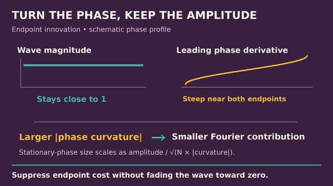
Simply tapering a wave’s amplitude near its endpoints helps control Fourier contributions, but risks destroying the lower modulus bound. The present construction instead changes curvature while keeping the main wave’s amplitude constant.
A small positive profile controls the relation between position and normalized frequency. Near endpoints, that profile becomes small, making the absolute phase curvature large. Stationary-phase estimates then suppress the endpoint contribution without requiring the wave itself to fade toward zero. This is the decisive separation between amplitude and Fourier cost.
The remaining short gaps must also be filled without crossing zero. On each gap, the proof interpolates amplitudes between nearby values close to one and builds a phase in three pieces. Short outer pieces join prescribed phase derivatives. A middle piece has its own assigned derivative interval, preventing many gaps from contributing strongly at the same normalized frequency.
Bounded phase adjustments match endpoint values exactly. Conjugate reflection completes the circle, with prescribed value one at the two reflection-fixed points. The construction matches the leading phase derivatives across joins. It does not require matching every full derivative of the resulting function, a stronger condition the argument does not need.
10. Controlling The Fourier Tail Through Boundary Cancellation
Deleting an infinite collection of tiny Fourier coefficients can still cause substantial error if their absolute sum is uncontrolled. The required estimate concerns the total exterior tail, not merely each coefficient separately.
Outside indices zero through , the combined phase has no stationary point. Its derivative stays quantitatively separated from zero because the leading phase derivatives remain inside a fixed subinterval of the allowed normalized range. Integration by parts therefore becomes effective.
The first integration produces endpoint terms. Continuity of and matching leading phase derivatives make adjacent terms cancel at every join, including the identified endpoints of the circle. A second integration yields coefficient decay strong enough to sum:
Summing gives total exterior mass of order . The constant depends on the auxiliary construction, which has already been fixed. This dependence matters when interpreting the absence of an effective convergence rate. The estimate supplies uniform projection accuracy, not a numerical recipe for selecting a practically adequate length at a chosen tolerance.
11. The Final Proof: Parseval, Discrepancy Rounding, And Exact ±1 Coefficients
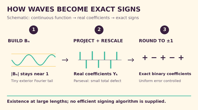
The retained real Fourier coefficients are rescaled into numbers between negative and positive one. Since has magnitude at least one and the rescaling factor is close to one, Parseval forces the average squared size of these numbers close to one. Their average shortfall from absolute value one is consequently small.
The defect-sensitive discrepancy lemma converts these numbers into exact signs while controlling the entire trigonometric sum. Independent nearest-sign choices would lack that guarantee. The lemma coordinates the rounding, using a finite sampling grid and a derivative estimate to extend control to every point of the circle.
| Component | Meaning And Scope |
|---|---|
| Projection | Removes exterior frequencies with a uniformly small error. |
| Parseval | Bounds the aggregate coefficient defect using nearly maximal energy. |
| Discrepancy rounding | Produces exact real signs with controlled uniform error. |
| Limit order | Fix auxiliary data first, then increase the integer length. |
| Output scope | Existence at each sufficiently large length, with no required shared sign prefixes. |
Finally, the proof chooses the auxiliary error small enough for the desired tolerance, then takes the length sufficiently large. Uniform approximation preserves both modulus inequalities. The conclusion is existential: no efficient general signing algorithm, effective convergence rate, or numerical application benchmark is supplied. Independently chosen signs at each length are allowed. The manuscript explicitly distinguishes this from the obstructed demand for ultraflat partial sums of one fixed infinite sequence.
For developers, the immediate value is a proof architecture worth studying, rather than a ready-made signal-design library. For researchers, the central advance asserted is the coordinated control of amplitude, endpoint curvature, and rounding error. As in our Courtade–Kumar coverage, theorem scope and verification scope deserve separate attention.
Littlewood polynomials make a precise test of what binary choices can achieve against continuous constraints. Follow Binary Verse AI for research explainers that trace the argument, its assumptions, and the evidence behind the headline.
What is a Littlewood polynomial?
A Littlewood polynomial is a polynomial whose coefficients are exclusively +1 or −1. The paper studies whether such real-coefficient polynomials can maintain an almost constant magnitude on the complex unit circle.
Why is the square root of N the ideal magnitude?
Parseval’s identity shows that the average squared magnitude of a length- Littlewood polynomial on the unit circle equals . Therefore, is the natural magnitude scale.
What is the difference between flat and ultraflat Littlewood polynomials?
Flatness keeps the magnitude between fixed positive multiples of . Ultraflatness is stronger: both normalized maximum and minimum approach one uniformly as the length increases.
What exactly does OpenAI’s proof establish?
The manuscript presents a proof that, for any fixed tolerance , every sufficiently large integer length admits a ±1 polynomial whose magnitude remains between and everywhere on the unit circle. The linked Lean notes document weaker statements, not this full uniform two-sided conclusion.
Why were real Littlewood polynomials harder than complex-coefficient polynomials?
Complex coefficients of modulus one permit continuously adjustable phases. Real Littlewood polynomials permit only two coefficient choices, +1 and −1, making uniform magnitude control substantially harder.
How does OpenAI’s proof convert oscillating waves into exact ±1 coefficients?
The proof constructs an almost-flat continuous function, controls its Fourier coefficients, and uses Parseval’s identity to bound their aggregate magnitude defect. A discrepancy rounding lemma then converts the relevant real coefficients into exact signs while controlling the uniform error.
Does the proof provide an explicit efficient algorithm or one fixed infinite sign sequence?
No efficient general sign-selection algorithm or effective convergence rate is established. The theorem permits independently chosen signs at each sufficiently large length and does not assert that all polynomials arise as partial sums of one fixed infinite sequence.