
A weight with a hundred binary digits can derail an algorithm that looks efficient on small numbers. Mean payoff games have carried that trap for decades: compact inputs can encode enormous numerical work. OpenAI’s September 25, 2026 manuscript presents a deterministic algorithm that computes every zero-threshold winner in quasipolynomial time measured against the complete binary input length. Reductions also recover exact values and optimal memoryless strategies.
The advance concerns a worst-case mathematical guarantee. Polynomial time remains open, and the manuscript supplies no practical speed benchmark. Its central trick is to classify potential-function boundaries without climbing through an enormous numerical range, using stationary pivots and carefully reweighted proof witnesses.
Table of Contents
1. What Are Mean-Payoff Games? The Infinite Game Behind the Proof
A finite directed graph has vertices, each owned by Max or Min, and every vertex has an outgoing edge. Its owner chooses the next move. Each edge carries a signed integer weight. Max wants a large long-run average; Min wants a small one. For the infinite edge sequence , the payoff is:
Here counts moves. The limit inferior captures the lowest asymptotic average when ordinary averages fail to converge. The zero-threshold question asks whether Max can guarantee a nonnegative payoff against every opposing strategy, including strategies using the entire history.
| Aspect | Verified Scope |
|---|---|
| Input | Finite directed graph; signed integer weights encoded in binary |
| Choices | Max and Min own vertices; self-loops and parallel edges are allowed |
| Main output | All starting vertices where Max guarantees nonnegative liminf average |
| Complexity | Deterministic quasipolynomial bit time in complete input length |
| Extensions | Exact rational values and globally optimal positional strategies |
For a mean payoff games example, let Max’s vertex A offer a weight-zero edge to B or C. At Min’s vertex B, self-loops have weights +2 and −1. Vertex C has only a +1 self-loop. Min makes B worth −1, so Max chooses C and obtains value +1 from A. The single initial zero disappears from the long-run average.
2. Why Mean-Payoff Games Resisted Faster Algorithms for Decades
Classical positional determinacy says both players have optimal strategies depending only on the current vertex. This places the threshold decision problem in : each side has a polynomially checkable strategy certificate. It does not give a fast method for finding those certificates.
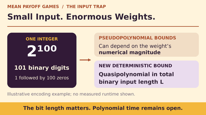
Earlier pseudopolynomial methods could depend polynomially on the largest absolute weight. A weight such as takes only 101 binary digits, while work proportional to its magnitude is astronomical. That mismatch is the binary-weight bottleneck in mean payoff games complexity.
Quasipolynomial parity-game algorithms did not automatically fix it. Parity games reduce to mean-payoff games with large but succinctly encoded weights. That reduction points toward the harder numerical problem, so reversing its algorithmic implication is invalid.
The challenge persists despite the graph being finite. Strategies generate infinite plays, and the algorithm must classify all possible opposition without listing those plays. Positional certificates compress the answer, but searching the space of possible policies can still be expensive.
Computational measures need the same care elsewhere: space simulation bounds measure memory, while quantum query complexity counts input accesses. Here the accounting covers deterministic bit operations, including arithmetic.
3. What OpenAI’s Deterministic Quasipolynomial-Time Proof Establishes
Theorem 1.1 in the deterministic mean-payoff games manuscript returns the complete winning set, rather than answering for one selected start. Let denote the full explicit binary encoding of vertices, ownership, edge endpoints, and weights. The bound is:
Quasipolynomial growth lies beyond a fixed polynomial bound, yet below familiar exponential growth in input length. The theorem includes preprocessing, recursion, exact arithmetic, and the entire output. Random success is unnecessary.
OpenAI describes the broader release as results produced by an internal frontier model in its mathematics release announcement. That attribution does not establish independent validation of every theorem. The published Lean scope documentation covers the related randomized algorithm and a finite counterexample to an older optimization step. It does not document complete formal verification of this deterministic theorem. As with proof formalization in Lean, the checked statement and its scope matter.
4. The First Proof Step: Perturbing Weights to Eliminate Zero Cycles
Zero-weight cycles obstruct the comparison machinery. The proof transforms each original edge weight using:
A simple cycle has length between 1 and . If its original integer sum is , its transformed sum is . For , this is positive. For , it is negative. No simple cycle now has zero sum.
The transformation deliberately makes originally zero cycles positive. It preserves the distinction needed for the nonnegative threshold, rather than preserving every cycle’s original sign literally. For , a two-edge cycle totaling −1 becomes −2; one totaling zero becomes +2. The numerical weights grow, but their binary descriptions grow modestly. Positional determinacy and cycle arguments carry the resulting threshold partition back to the original game.
5. Potential Functions, Finite Boxes and the Comparison Theorem
Assign each vertex an integer potential . The operator evaluates the best or worst transformed edge-plus-successor potential according to ownership:
A finite box restricts each coordinate between a lower endpoint and an upper endpoint . Clipping means replacing any proposed coordinate outside that interval by the nearest endpoint.
A subsolution satisfies wherever . A supersolution satisfies wherever . The excluded boundaries are essential: neither condition is imposed everywhere.
Two operator properties make translations useful. Increasing every input coordinate cannot decrease any output coordinate. Adding the same integer to every coordinate adds that integer to every output as well. This common-shift invariance lets the proof relocate a witness without changing the local inequality it must satisfy before clipping.
Lemma 2.1 imports the companion paper’s finite-box comparison theorem and basic iteration. For this perturbed operator, there is a unique clipped fixed point , and every such pair satisfies . Monotonicity alone would not establish uniqueness. The cycle hypothesis matters. Basic iteration finds , but on a wide box it can require work proportional to numerical width. The new algorithm avoids that cost.
6. How a Wide Potential Box Separates Winners From Losers
Let be the largest absolute transformed weight. Choose as the smallest power of two at least . Proposition 2.2 places every coordinate of the solution in one of two disjoint bands:
Why can nothing remain in the middle? At an interior coordinate, an edge attains the exact potential equality. Following such edges must reach a boundary within moves. Repeating a vertex first would create a tight simple cycle with transformed sum zero, which the perturbation forbids. Each edge changes potential by at most , giving the distance bound.
The cycle argument also controls arbitrary nonperiodic opposition. Remove simple cycles from any finite play prefix. What remains has fewer than n edges, so its possible negative contribution stays bounded independently of the prefix length. Dividing by a growing length makes that transient contribution vanish.
In the upper band, Max selects edges satisfying the subsolution inequality. At Min vertices every edge satisfies it. These choices remain in the band, and potential differences telescope around cycles. Original cycle sums are nonnegative. The lower band gives Min the dual guarantee, with original upper limiting average at most . Thus the bands identify winners without requiring an explicit wide-box solution.
7. Witnesses, Boundary Labels and Translation Into Narrower Boxes
The recursion asks for plus and minus labels that satisfy many potential certificates simultaneously. In a width- box, a Max witness is a subsolution whose support, the coordinates above their lower boundaries, has total positive rational mass at most one. Min uses supersolutions, coordinates below their upper boundaries, and separate masses.
A witness claims coordinates within of its favorable boundary. Opposing claims cannot coincide because comparison orders every subsolution below every supersolution. Initially each coordinate receives mass on both sides, so every support qualifies and the box solution’s claims settle every winner.
Support mass is an accounting constraint, not a probability of winning. There is no random sampling here. Nor does restricting a witness support delete vertices or edges from the game. Each recursive call retains the original graph and changes the box and mass parameters.
For recursion, a pivot sits near the box center. A Max witness’s peak is ; its gap at a coordinate measures distance below that peak. Translate the whole vector by one common amount, then clip at the narrower box’s bottom. Its surviving support is exactly the coordinates with gap below the child width. Near-peak coordinates become upper-boundary claims. Min uses the dual construction. Supports only shrink, preserving eligibility under unchanged masses. Witnesses are proof objects, never enumerated by the executable algorithm.
8. Inside OpenAI’s Deterministic Recursion: Downward and Upward Pivot Passes
For , set center , movement cap , narrow width , and step . Each update uses one child’s entire label vector simultaneously.
| Pass | Child Masses | Movement and Protection |
|---|---|---|
| Downward | Max masses unchanged; Min masses multiplied by | Minus-labelled coordinates move down by , capped at . Max peaks stay fixed. |
| Upward | Max masses multiplied by ; Min masses unchanged | Plus-labelled coordinates move up by , capped at . Min peaks stay fixed. |
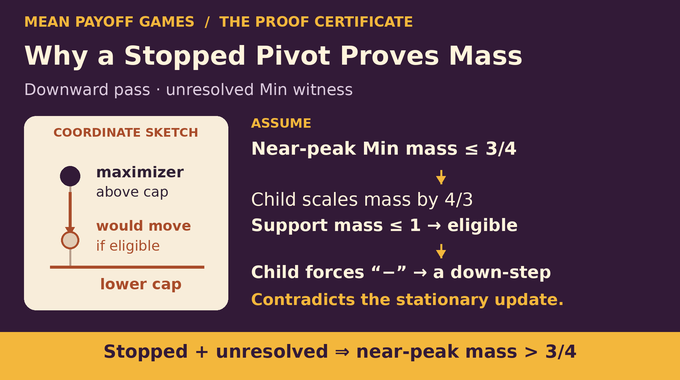
The protected peak explains safety. In the downward pass, every Max gap at most becomes a child claim and receives plus, so that coordinate stays still. Coordinates farther away move by at most and cannot overtake the peak. Min receives the symmetric protection upward.
The algorithm records downward marks where the stopped pivot lies more than below the center, and upward marks where the final pivot lies more than that distance above it. Peak protection proves that these marks cannot overwrite a claim belonging to the opposing witness type.
The final stationary call is decisive. Suppose a Min witness still claims an unmarked coordinate after the downward pass. Its maximizing pivot deviation lies above the lower movement cap. If its near-peak support had original Min mass at most , multiplying by would leave it eligible. The child would force minus at a maximizer, requiring movement. Stationarity contradicts that possibility.
Consequently the unresolved near-peak mass exceeds . This Min certificate survives the upward pass because its near-peak set can only grow. The upward stopping call supplies the matching Max certificate. These inequalities turn stopped motion into usable evidence.
9. Mass Reweighting: Why Every Unresolved Witness Eventually Disappears
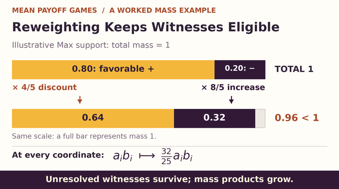
A child of width now labels the certified near-peak sets. They fall within its claim margin, so every unresolved witness gets its favorable label on mass greater than . These provisional labels guide reweighting, rather than directly settling the parent’s claims.
At a plus label, multiply Max mass by and Min mass by . At minus, reverse those multipliers. For an unresolved Max support , write for the provisional plus coordinates. Its new mass obeys:
The Min calculation is symmetric. Unresolved witnesses therefore remain eligible in the continuation on the original box. Meanwhile every coordinate’s mass product grows by , independently of its label.
Starting from product , only logarithmically many such increases fit before every product exceeds one. At that base case each coordinate is too heavy for at least one witness type, allowing a direct safe label. Witnesses need not literally disappear together: the precise progress measure is growing mass products alongside shrinking widths.
10. Why the Recursion Is Correct and Its Running Time Is Quasipolynomial
Correctness uses induction on a rank combining logarithmic width with the remaining mass-growth budget. Pivot-pass children increase products by ; the continuation increases them by . The provisional child alone preserves masses, but halves width. Every child decreases the rank.
Marked coordinates receive safe overrides: downward marks cannot contain Max claims, and upward marks cannot contain Min claims. Every remaining claim belongs to a witness preserved by reweighting, so induction makes the continuation respect it. The guarantee holds simultaneously for all witnesses.
At small width, below 4096, direct iteration becomes safe: it needs at most one plus operator evaluations. Each evaluation scans the explicit edges. This is where the executable procedure actually evaluates the game operator. The large-width recursion manipulates labels and exact mass parameters instead of searching for witness vectors.
Each pass uses only linearly many child calls in . A branch has polynomial depth in , but only mass-budget decreases. Crucially, only one child preserves that budget. Counting where the other branches occur gives the quasipolynomial bound. Integer coordinates and rational masses retain polynomial bit length; floating-point approximations are unnecessary.
This is exact worst-case complexity, not an approximation ratio like the factor-two superstring guarantee, or a competitive ratio like the randomized k-server bound. Those guarantees answer different algorithmic questions.
11. Exact Game Values, Optimal Positional Strategies and the Remaining Open Problem
Fixing both optimal positional strategies eventually repeats a simple cycle. Hence each exact value is rational with denominator at most . To test threshold , replace weights by . Polynomially many threshold queries narrow each value to an interval containing only one eligible rational.
Strategies require additional care. An edge between equal-value vertices can still be a losing choice if it traps play in an inferior cycle. The paper tests edge restrictions while preserving the entire value vector. Max and Min are recovered separately from fresh copies of the original game, yielding strategies optimal from every vertex against history-dependent opposition.
Direct corollaries decide prescribed-credit one-resource energy games and compute minimum winning credits, including infinity when no finite credit works. Other classical reductions give tropical feasibility and tropical-rank tests at fixed corank. These are precisely scoped consequences, not a general polynomial-time tropical optimization result.
Finite minimum energy credits are bounded by , where is the largest absolute original weight. That bound supports binary search over credit values, rather than an array whose size depends on their numerical magnitude.
For developers, implementation and benchmarking remain work to do: the proof establishes no production speedup. The difference between a complexity theorem and a usable solver also matters in exact three-machine scheduling and maximum cardinality matching. Mean payoff games now have a deterministic quasipolynomial construction in this manuscript; polynomial time remains the next question. Follow Binary Verse AI for research explainers that trace the argument from its original bottleneck to its actual guarantee.
What is a mean-payoff game in game theory?
A mean-payoff game is a two-player, zero-sum game on a finite weighted directed graph. Players choose edges indefinitely. Max seeks a large long-run average edge weight, while Min seeks a small one. The paper determines which starting vertices let Max guarantee a nonnegative liminf average.
How is the mean payoff calculated?
Average the weights of the first T moves, then take the limit inferior as T grows without bound. The limit inferior handles sequences whose averages do not converge. This is the long-run payoff of an infinite path, rather than the expected payoff of a one-shot matrix game.
Why were mean-payoff games difficult to solve efficiently?
Earlier pseudopolynomial methods could depend on the numerical magnitude of edge weights. An enormous integer can have a short binary encoding, so those methods can require exponential time in input length. The new manuscript establishes a quasipolynomial bound in the complete explicit binary input size.
Did OpenAI prove that mean-payoff games can be solved in polynomial time?
No. The manuscript gives a deterministic algorithm using bit operations, where L is the complete binary input length. This is quasipolynomial time. It does not establish a polynomial-time algorithm.
Does OpenAI’s algorithm compute optimal strategies as well as winners?
Yes. The main theorem computes the complete zero-threshold winning set. Corollary 7.1 then uses threshold queries and strategy self-reductions to compute exact rational values and globally optimal positional strategies for both players within the same quasipolynomial bit bound.
Has OpenAI’s deterministic mean-payoff games proof been formally verified?
The published Lean documentation covers a related randomized quasipolynomial algorithm and a finite counterexample to an older optimization procedure. That documentation does not establish complete Lean verification of the deterministic theorem. The manuscript’s mathematical proof and the documented formalization scope should be distinguished.