
A polynomial equation can have just one possible solution and still defeat every universal decision algorithm. That is the striking consequence of OpenAI’s September 24, 2026 paper on the single fold Diophantine conjecture. Its main theorem gives every recursively enumerable set a polynomial representation with exactly one complete natural-number witness for each member and none for nonmembers.
The proposed mechanism connects elliptic curves, Pell equations and encoded computations. The difficult part is preserving uniqueness through every auxiliary calculation. OpenAI’s mathematics release provides the publication context. Its formalization documentation separately identifies what Lean establishes.
Table of Contents
1. What Is the Single Fold Diophantine Conjecture?
A Diophantine representation translates membership in a set into polynomial solvability. The input is a tuple of natural numbers, and additional natural numbers supply a witness. Here, natural numbers include zero. Integer coefficients may be negative even though witnesses cannot be.
A recursively enumerable set has a program that accepts precisely its members. On a nonmember, that program may continue forever. Theorem 1.1 of Single-fold Diophantine representations states that every such set of finite natural-number tuples has a single-fold representation.
| Question | Paper’s Answer |
|---|---|
| Main theorem | Every recursively enumerable subset of has a single-fold polynomial representation, for . |
| Witness count | Exactly one complete tuple for a member, zero for a nonmember. |
| Coefficient domain | Integer polynomial coefficients. |
| Witness domain | Natural numbers, including zero. |
| Arithmetic mechanism | Rank-one elliptic curve heights supply a uniquely represented cutoff for Pell equations. |
| Manuscript date | September 24, 2026. |
| Verification scope | Reported Lean formalization of the main representation theorem; the undecidability consequence is not separately formalized. |
For a member, exactly one entire witness tuple makes the polynomial vanish. For a nonmember, no tuple does. Uniqueness includes variables introduced to express division, comparisons and rational arithmetic. One preferred answer accompanied by infinitely many alternative certificates would fail the requirement.
This is stronger than merely recognizing solvable equations. It specifies how many explanations of membership the polynomial can admit, including every component normally hidden inside a subsidiary calculation.
The polynomial is fixed for the chosen set. Its inputs vary, while its finite witness length stays fixed. This belongs to the computability landscape explored in our Turing degrees analysis.
2. Why the MRDP Theorem Did Not Solve the 1974 Conjecture
The Davis–Putnam–Robinson–Matiyasevich theorem, completed in 1970, already gave recursively enumerable sets polynomial representations. It settled Hilbert’s tenth problem negatively: no algorithm decides solvability for every integer polynomial equation in its original setting. It did not control witness multiplicity.
Matiyasevich’s 1974 work achieved unique complete witnesses when the representation could use exponentiation. It also formulated the remaining polynomial-only problem. The 52-year interval refers to that 1974 formulation and this 2026 manuscript.
Replacing an exponential relation by an ordinary polynomial relation can introduce many auxiliary solutions. A proof must eliminate those extra choices, rather than merely preserve existence. This explains why ordinary Diophantine representability did not finish the Matiyasevich single-fold conjecture.
The domain also matters. Binary Verse AI’s coverage of Hilbert’s tenth problem over the rationals concerns a different solvability question. Rational coordinates inside this construction do not change its final natural-number witness domain.
3. The Previous Barrier: Why Exponentiation Lost Its Unique Witness
Pell equations offer a classical route to exponentiation. Their positive solutions form sequences indexed by natural numbers, and certain coordinates grow exponentially. Congruences can identify the desired index modulo a large number.
The catch is that congruences specify a residue class. They do not distinguish one index from every larger index with the same residue. A cutoff must force the relevant indices into a range where the residue determines them exactly.
Simply allowing an arbitrarily large cutoff creates new witnesses. Defining it through exponentiation would also assume the operation the polynomial construction is trying to recover. The cutoff therefore needs its own polynomial representation with unique complete witnesses.
The paper supplies a function with carefully intermediate growth. Its upper bound excludes unwanted Pell indices. Its lower bound admits the intended solutions. Both bounds matter: a tiny cutoff could give uniqueness by excluding every solution, which would prove nothing useful.
4. How the OpenAI Proof Preserves Uniqueness at Every Step
Lemma 2.2 makes uniqueness compositional. Once a function’s input fixes its output and every internal variable, its output can feed another uniquely represented function without creating choices.
Comparisons require the same discipline. To encode that one integer expression is at least another, introduce their nonnegative difference. For strict inequality, subtract one as well. Each successful comparison determines its slack uniquely. Division similarly uses a quotient and a remainder smaller than the positive divisor.
Disjoint cases need special care. Only one branch may be active, and every variable local to an inactive branch is forced to zero. Otherwise an unused slope or denominator could vary freely and destroy single-foldness.
Rational numbers receive reduced, positive-denominator codes. The modular inverse used to certify reducedness is restricted to one residue interval, making that certificate unique too. Appendix B tracks the complete tuple through nested calls. The proof’s bookkeeping is part of its mathematical content, not optional implementation detail.
For example, allowing both one-half and two-quarters as coordinate codes would immediately create different witnesses for the same rational point. Reducedness removes that ambiguity. Restricting the inverse certificate removes a second ambiguity that ordinary fraction normalization alone would leave behind.
5. Why the Chosen Elliptic Curve Changes the Problem
The arithmetic construction uses the curve
Its rational-point group has rank one. Its torsion subgroup consists exactly of the identity at infinity and the three affine points with coordinates , and . Appendix A proves these facts through descent and a torsion argument.
Consequently every rational point has a unique expression , with an integer index , a fixed generator modulo torsion , and a torsion point . The rank concept also appears in our Birch and Swinnerton-Dyer explainer, although this proof needs only one specific curve’s arithmetic.
The construction removes sign and torsion ambiguity. Among torsion translates it chooses the point with greatest x-coordinate, then selects the sign with positive y-coordinate. This leaves exactly one representative for every positive absolute index.
The curve functions as an indexed arithmetic structure. Its role differs from the automorphic correspondence discussed in elliptic curve modularity.
6. How Canonical Heights Create a Strictly Increasing Sequence
For a reduced rational coordinate, its integer height is the larger of its absolute numerator and positive denominator. The logarithm of this height measures arithmetic size. It is not simply the coordinate’s magnitude.
Elliptic curve canonical height grows exactly quadratically under integer multiplication of a point. Ordinary logarithmic coordinate height differs from twice canonical height by a uniformly bounded amount.
After multiplying representatives by one fixed, sufficiently large even integer, the paper obtains integer heights satisfying
Here , , and bounds the error independently of the index. The fixed multiplier enlarges the quadratic coefficient without enlarging that error bound. Successive quadratic gaps then dominate possible errors, making the sequence strictly increasing.
This is the useful feature of the elliptic curve canonical height: predictable arithmetic growth with bounded noise. The polynomial system calculates rational-point operations and integer heights. Real logarithms justify the comparisons in the proof and are not additional polynomial variables.
7. The Key Breakthrough: Selecting Exactly the Squared Index
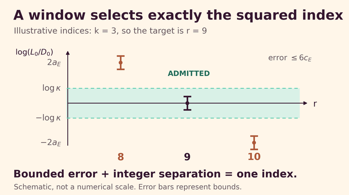
First select the unique representative whose index satisfies
For a second representative with positive absolute index , form
Doubling the first point supplies the doubled index. Adding or subtracting the fixed generator supplies neighboring heights, whose maximum selects the larger neighbor. These are fixed point operations, so the system need not quantify the indices themselves.
Taking logarithms in the analysis gives
The quadratic term in the second index cancels. Choose a fixed integer so that the bounded-error interval around zero fits inside the window, while every incorrect integer index falls outside it. The actual polynomial conditions are
These hold exactly when . For example, at , the selector admits index nine and excludes eight and ten. The reason is the proven gap between integer indices, rather than numerical approximation to a logarithm.
8. Building the Intermediate-Growth Function
Proposition 4.2 defines , using the unique input-scale index and the squared-index selector. Every input, including zero, fixes one output and one complete auxiliary tuple.
The input bracket makes the square of the selected index comparable to the logarithm of the input. Squaring that index again in the height estimate makes the output’s logarithm comparable to the square of the input’s logarithm.
For some fixed positive and all sufficiently large natural inputs, the paper proves
Thus the output eventually grows faster than every fixed power of the input, while remaining below the input raised to itself. These are asymptotic statements with fixed thresholds, not assertions about every small input.
The function’s graph is polynomial even though its growth analysis uses logarithms. Fixed integers and rational-point codes enter the equations. Real-valued estimates establish that those fixed choices work. This distinction prevents the construction from quietly importing transcendental operations into its Diophantine representation.
9. How Two Pell Equations Recover Exponentiation
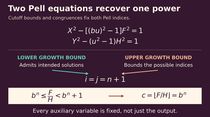
Proposition 5.2 applies the growth function to two Pell equations, with parameters and . Here is the power’s base, its exponent, and the proposed output.
The scale is prescribed by a fixed polynomial expression in those three quantities. It is not an independently selectable large number. Both Pell coordinates must lie below , and congruences require their indices to match .
The upper growth bound makes the indices smaller than the relevant modulus range. The congruences therefore fix both indices exactly. The lower bound proves that the intended coordinates really fit under the cutoff.
Finally, dividing the coordinate from parameter by the coordinate from parameter gives an integer quotient. The ratio lies at least at and strictly below , forcing .
The argument then fixes the scale, both Pell solutions, every quotient, remainder and comparison slack. That is single-fold exponentiation, including its internal arithmetic witnesses, rather than just a unique displayed output.
10. How Lucas’s Theorem Encodes Binary Digits
The next relation tests binary containment: every position containing a one in the first number must also contain a one in the second. For example, binary 101 is contained in 1101, but binary 110 is not.
Lucas’s theorem modulo two identifies this condition with the binomial coefficient being odd. The paper derives the parity rule by factoring the binomial expansion over the two-element field.
To express the test polynomially, choose a power-of-two base larger than every relevant binomial coefficient. Expanding the base plus one to the required exponent packs the coefficients into separate digits without carries. Exponentiation supplies the packed integer and the position of the desired digit.
Two uniquely determined divisions extract that digit. A final equation checks oddness with its unique parity quotient. Every power call retains its complete auxiliary tuple. The resulting bit mask can restrict permitted positions throughout an encoded computation, while preserving the uniqueness already established arithmetically.
11. From a Halting Computation to One Polynomial Witness
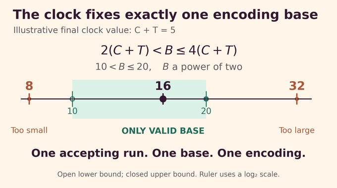
A deterministic counter machine accepts precisely the target set. Its counters support increment and conditional decrement instructions. The proof packs successive configurations into digits of finitely many integers, using a power-of-two base.
Masks record states and branches. Polynomial identities enforce transitions, while binary containment enforces zero tests and allowed counter digits. The halt state occurs only in the final recorded configuration, preventing padded histories.
The accepting run is unique, but its encoding would not be unique if the base remained free. A clock fixes that too. If the run takes instructions and is the prescribed initial bound, the base must be the unique power of two satisfying
This is a representation argument, whereas our Turing-machine time-space explainer concerns simulation resources. Here, arbitrary runtime is stored in integer sizes, not a runtime-dependent number of variables.
Encoding a halting problem also underlies Turing-complete fluid constructions. Here the receiving object is a polynomial system, and every part of its computational certificate must be unique.
After expanding every arithmetic call, the proof adds the squares of all polynomial constraints. Their sum vanishes exactly when each constraint vanishes, without introducing another variable. A member supplies one complete witness. A nonmember supplies none.
12. What the OpenAI Proof Establishes and Its Limitations
The finite-fold Diophantine conjecture follows immediately: one witness is finite. Corollary 1.2 also establishes undecidability with at most one natural-number solution, even with fixed existential bounds on degree and variable count. Coefficients can vary between inputs.
This differs from the runtime questions in our exponential time hypothesis analysis. Undecidability rules out a universally terminating correct decision procedure for the promised class.
| Aspect | Exact Scope |
|---|---|
| Finite-fold consequence | Established by the stronger single-fold assertion. |
| Undecidability promise | Zero or one complete natural-number solution; no universal decision algorithm, even for some fixed variable and degree bounds. |
| Explicit construction | Some fixed arithmetic constants, the final coefficients and numerical degree and variable bounds are not supplied. |
| Other domains | No corresponding single-fold theorem with unrestricted integer or rational witnesses is asserted here. |
| Practical performance | The result supplies no demonstrated solver benchmark or practical equation-generation procedure. |
The promise permits zero solutions as well as one. Under an exactly-one-solution promise, existence would already be guaranteed. The corollary instead asks which of the two possibilities occurs, and shows that uniqueness does not make that decision universally computable. It does not prevent solving individual equations or restricted subclasses.
OpenAI’s Lean scope documentation reports formalization of the main representation theorem and explicitly excludes a separate formalization of the undecidability consequence. This article does not independently rebuild or audit that code. Formal checking and independent mathematical review answer different questions.
Witness domains remain essential, as our existential theory of the reals explainer illustrates. Changing the permitted numbers changes the solvability problem.
The single fold Diophantine conjecture result connects unique arithmetic certificates with unique computational histories. For developers, its practical lesson is about guarantees: uniqueness alone supplies no general decision procedure. Follow Binary Verse AI for research explainers that trace the argument and identify exactly what its evidence supports.
What is a single-fold Diophantine representation?
It is a polynomial representation in which every member of the represented set has exactly one complete tuple of natural-number auxiliary witnesses, while every nonmember has none. Uniqueness counts every auxiliary variable.
Why didn’t Matiyasevich’s theorem already prove the single-fold conjecture?
The 1970 MRDP theorem established polynomial Diophantine representability without restricting witness multiplicity. Matiyasevich’s 1974 construction achieved unique witnesses with exponentiation permitted. Obtaining polynomial-only uniqueness required an additional argument.
Why does the OpenAI proof use elliptic curves?
The chosen rank-one curve supplies an integer-indexed family of rational points whose logarithmic coordinate heights grow quadratically with uniformly bounded error. That structure permits exact index selection and supplies the missing uniquely represented growth cutoff.
Does the single-fold proof also settle the finite-fold Diophantine conjecture?
Yes, as a consequence of the paper’s stronger theorem. A representation with exactly one complete witness for each member necessarily has finitely many witnesses for every input.
Can a Diophantine equation still be undecidable if it has at most one solution?
Yes, in the algorithmic sense stated by Corollary 1.2: no algorithm can always halt and correctly decide solvability for every equation promised to have zero or one natural-number solution, even with some fixed bounds on variable count and degree. Undecidability concerns that class of inputs, rather than a claim that every individual equation resists analysis.
Does the proof apply to Diophantine equations over integers or rational numbers?
The theorem concerns sets of natural-number tuples and auxiliary witnesses in the natural numbers, including zero. Its polynomials have integer coefficients, and rational points appear inside the construction. It does not directly establish corresponding single-fold results with unrestricted integer or rational witnesses.
Has the single-fold Diophantine proof been formally verified in Lean?
OpenAI’s scope documentation reports a Lean formalization of the main single-fold representation theorem. The undecidability consequence is not separately formalized. This article does not independently rebuild or audit the formalization, and formal checking should not be confused with independent mathematical peer review.