
A graph can reveal one perfect pairing quickly while concealing how many others exist. Counting perfect matchings asks for that hidden population, and arbitrary graphs have resisted a general randomized approximation guarantee for decades. OpenAI’s September 23, 2026 paper supplies a fully polynomial randomized approximation scheme, or FPRAS: an estimate with selectable relative accuracy and failure probability, obtained in worst-case polynomial bit time.
The advance comes from rebuilding the sampling problem. The proof creates an enlarged weighted graph, controls the cost of unmatched vertices, and couples matching coordinates across nearby distributions. It escapes a specific exponential obstruction to earlier chains. Here is how that machinery turns samples into a count, and what the theorem actually guarantees.
Table of Contents
1. Counting Perfect Matchings: What Is the Problem?
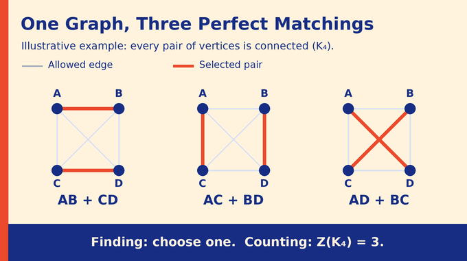
Let be a finite simple undirected graph. Vertices represent objects, edges represent allowed pairings, and a perfect matching covers every vertex exactly once. Write for the collection of perfect matchings. The target is:
On the complete four-vertex graph , label vertices A, B, C, and D. Its three possibilities are AB with CD, AC with BD, and AD with BC. Finding one answers feasibility. Counting asks for all three without necessarily listing them. Our maximum cardinality matching explainer addresses the related optimization task.
| Primary Paper | OpenAI, September 23, 2026 manuscript. |
|---|---|
| Input | Any finite simple undirected graph, without a density or expansion promise. |
| Output | A nonnegative rational estimate with prescribed relative error and confidence. |
| Zero Case | No perfect matching means zero on every execution. |
| Time Guarantee | Polynomial bit time in input length, inverse relative error, and logarithmic inverse failure probability. |
| Practical Evidence | The manuscript establishes an algorithmic bound, without competitive runtime benchmarks. |
2. Why Counting Perfect Matchings Is Computationally Hard
Edmonds’s algorithm establishes polynomial-time existence testing in general graphs. Exact counting is #P-complete even for bipartite graphs, where it equals the permanent of a zero-one bipartite adjacency matrix. The matrix specifies allowed left-to-right pairings, and each valid permutation contributes one.
Our permanent versus determinant analysis explains that algebraic connection. Here the issue is approximating a nonnegative count, rather than representing a polynomial by a determinant. #P-completeness does not itself forbid efficient randomized relative approximation.
Complete graphs have an exact shortcut: on vertices the count is . Choose a partner for the first vertex, then repeat on the remaining vertices. Arbitrary missing edges destroy this symmetry. Graphs with equally many vertices can have very different counts, including zero.
Special structure also matters: planar graphs admit polynomial-time exact counting through Pfaffian methods. The new theorem concerns unrestricted graphs, not a claim that every previously tractable case required approximation. The broader distinction between feasibility and counting also appears in counting common bases of two matroids.
A useful interpretation is flexibility: one valid pairing shows a system can function, while its count describes the number of available configurations. Turning that count into an application metric would still require a model connecting graph edges to real constraints. The theorem supplies no such domain assumptions.
3. The Previous Barrier: Why Earlier Matching Algorithms Could Not Solve the General Case
Jerrum and Sinclair obtained an FPRAS for counting all matchings, summed over every size. That is not enough to estimate the perfect-matching contribution accurately. If perfect matchings form an exponentially small fraction of the total, ordinary sampling rarely sees them.
Their perfect-matching approach required a polynomial bound on the ratio of near-perfect to perfect matchings. A near-perfect matching leaves exactly two vertices unmatched, called holes. Too many two-hole states can overwhelm the states being counted.
Jerrum, Sinclair, and Vigoda overcame this restriction for bipartite graphs, giving an FPRAS for the nonnegative permanent. They learned weights for classes of near-perfect states during gradual changes of edge weights.
However, Štefankovič, Vigoda, and Wilmes exhibited a precise general-graph obstruction. For the specified JSV-type chains, any weighting based on the hole pattern leaves either exponentially little perfect-matching mass or exponentially slow mixing. This is a limitation of those states and transitions, not an impossibility theorem for every sampler. OpenAI changes both.
4. What the OpenAI Proof Establishes: The FPRAS Theorem
Theorem 1.1 of the original perfect-matching paper gives a uniform classical randomized algorithm. For rational and , its estimate satisfies:
Here is relative error and is allowed failure probability. If the true count were 1,000, five-percent accuracy would mean a successful estimate between 950 and 1,050. This illustrates the guarantee, not measured performance.
Runtime is polynomial in input encoding length, , and . “Fully polynomial” explicitly charges for increasing accuracy, unlike merely fixing accuracy before an asymptotic analysis, a distinction relevant to our edit distance approximation guide.
The bound holds on every random execution, including unsuccessful ones. A deterministic matching-existence test handles zero before sampling. This makes the theorem stronger than an expected-runtime statement, while leaving exact counting’s complexity unchanged. Approximation guarantees must also be separated from optimization hardness, as in our Unique Games explainer.
Relative error is essential when counts vary enormously. An additive allowance based on every possible pairing could completely obscure a sparse graph’s actual count. Also, certain-zero behavior is one-directional: the stated theorem does not make every zero returned on an unsuccessful nonempty input an infeasibility certificate.
5. The Starting Point: Turning an Impossible Count Into Weighted Ratios
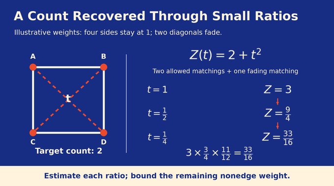
Assign each edge a positive activity . A matching’s weight is the product of its edge activities, and the partition function sums these products. Sampling chooses a matching with probability proportional to its weight.
Begin with the complete graph and unit activities, whose partition function is known. Keep input edges at weight one while gradually reducing the positive weights of nonedges. This annealing schedule avoids an abrupt jump into a distribution that might be difficult to sample.
Let denote the partition function at stage , with stages. The accounting telescopes:
A sample from one stage estimates the weight change at the next. Multiplying accurately estimated ratios recovers the final partition function. Nonedges retain tiny positive weights, so a separate bound controls their residual contribution to the target count. Nothing is rounded away without accounting for its error.
Think of dimming forbidden connections rather than deleting them immediately. Matchings using only allowed edges keep weight one. Every matching using a forbidden connection loses weight as the schedule advances. The final estimate still needs the proof that all surviving unwanted weight fits inside the error budget.
6. The Hole-Balance Argument: Controlling Near-Perfect Matchings
For activities , define the two-hole ratio . The numerator counts weighted perfect matchings after deleting vertices and . Large ratios indicate that freeing those vertices creates disproportionately many possibilities.
The proof maintains each row maximum between one-quarter and one. Vertex scaling accomplishes this: replacing an edge activity by multiplies every perfect-matching weight by the same factor , preserving its normalized distribution.
A bottleneck similarity measures the strongest weakest edge along paths from to , floored at one. For an even hole set , its pairing capacity is the maximum product of these similarities over pairings of its vertices.
Theorem 3.1 proves the following bound, where is the logical vertex count and :
This converts pairwise balance into control of every even hole set. The capacity is an analytical tool, not something the algorithm computes by enumerating all pairings.
That distinction prevents a hidden exponential subroutine. The algorithm learns pairwise quantities from samples. The theorem handles the many possible larger hole patterns collectively, ensuring that adding auxiliary edges remains affordable without checking those patterns individually.
7. Weighted Subdivision and Tree Bags: Constructing a Better Sampling Space
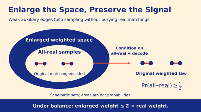
Replace every logical edge with a carefully weighted odd-length path. Matching its internal vertices has two patterns: one uses both original endpoints, while the other uses neither. Their weight ratio equals the logical edge activity. Thus real-path perfect matchings correspond bijectively to logical perfect matchings, with one common weight multiplier.
Threshold connectivity organizes these paths into a hierarchy. Overlapping vertex groups, called bags, receive weak auxiliary clique edges. Bags are indexed by a tree, and each vertex belongs to one bag or two adjacent bags.
These additions create useful switching opportunities, but they must not bury the original matchings under auxiliary ones. The hole bound proves that, under balance, the partition function grows by less than a factor of two. Consequently, a weighted sample uses only real edges with probability at least one-half.
Edge portions are revealed as real, virtual, or designated probes. With the inflation factor and the construction’s polynomial parameter, the event “probe for , all other edges real” has probability . That exact identity turns observable events into the hole estimates required for balancing.
8. Alternating Cycles and the Two-Coordinate Energy Inequality
Overlay two perfect matchings. After common edges are removed, the remaining components are even cycles whose edges alternate between the two matchings. Exchanging the two patterns on a cycle preserves the product of their weights.
The pair kernel combines cycle exchanges with two-edge switches and changes of edge color. Colors distinguish parallel edges supplied by different bags. Within one common target distribution, cycle exchanges are always accepted because their product weight is unchanged.
The proof divides cycle polygons into four-corner cells adapted to bag labels. Relevant edge weights remain comparable, allowing the associated local operations to be charged at polynomial cost. Its signed identity also uses conversions along long arcs. Those conversions are algebraic comparisons, not necessarily legal individual chain transitions.
Dirichlet energy measures the average squared change of a numerical observable in one stationary update. Theorem 6.1 bounds the variance of an observable on the first matching by the energy of an additive observable on both. Independent cycle exchanges control errors caused by differing matchings outside a chosen arc. This replaces the failed traditional chain argument with a comparison tailored to the enlarged space.
Intuitively, a quantity cannot vary greatly across the relevant distribution while remaining almost unchanged under all the useful updates. The challenge is proving that statement with only polynomial losses, despite extremely unequal weights and dependence on the surrounding matching.
9. From Energy Bounds to Rapid Mixing: The Key Technical Breakthrough
A restricted Poincaré inequality controls only a specified family of observables. Rapid mixing needs a spectral-gap bound for arbitrary functions of the full state. Moving between these statements requires another argument.
The sampler builds a ladder of nearby weight tiers by clamping activities to expanding common intervals. Adjacent tier distributions differ by at most a factor of two at any matching. The bottom tier has unit activities, permitting exact counting and ideal sampling through tree dynamic programming.
Many independent matching coordinates occupy each tier. Updates couple coordinates on adjacent tiers, while bottom coordinates can refresh. The stationary law is their product distribution. Across unequal tiers, even cycle exchanges require the appropriate Metropolis acceptance test.
An ordered orthogonal decomposition separates fluctuations into coordinate interactions. It ensures each relevant residual interaction is charged at most once. Replication then makes their combined coefficient small enough to absorb, yielding the full spectral gap. The proof uses copies per tier, with , where counts enlarged vertices. Polynomial does not mean small.
10. Recovering the Matching Count: Sampling, Error Control, and Polynomial Time
Marked samples serve two purposes simultaneously. All-real samples estimate the next partition ratio through their weight changes. Single-probe samples estimate two-hole ratios. Ratios of empirical averages cancel the unknown inflation factor, supplying the data for the next vertex-scale update.
Hoeffding concentration controls bounded observables. Sampling error, estimation error, and residual nonedge mass receive separate budgets. Stagewise ratio errors are small enough that multiplying the estimates preserves the final relative guarantee.
Each complete trial succeeds with probability greater than 0.9. Taking the median of independent trials reduces failure to the requested level with logarithmically many repetitions. The finite-bit implementation accounts for rational arithmetic and approximated random choices, rather than treating exact real numbers as free registers.
Crucially, the sampler’s time bound does not depend on successful balancing. Balance proves statistical usefulness along successful histories. Unconditional parameter caps bound every history’s runtime. This separation prevents an inaccurate estimate from triggering unlimited work, a concern also relevant to the randomized guarantees in our Subset Sum analysis.
For developers, the proof therefore specifies more than a stopping rule for a random walk. Initialization, graph expansion, storage, sampling precision, and arithmetic all contribute to the complexity account. Testing one apparently well-mixed trajectory would not establish any of those worst-case guarantees.
11. What the Proof Changes, and What It Does Not
| Approximate Counting | Relative accuracy with controlled failure probability, not exact enumeration. |
|---|---|
| Sampling | Feasible outputs on every feasible run, with controlled total-variation distance from uniform. |
| Further Families | Fixed-size matchings and edge subsets with prescribed vertex degrees, on explicitly listed simple unweighted hosts. |
| Deployment | No demonstrated practical speedup or competitive implementation benchmark in the supplied paper. |
Section 10 transfers the guarantee through counting reductions with known constant multiplicities. Its sampling result is closeness in total variation, not exact uniformity or a pointwise relative probability bound for every object. It reports infeasibility exactly for empty families.
Total variation bounds the discrepancy in probability assigned to any event. It can still permit large relative errors for exceptionally rare individual matchings. That is why “approximately uniform” needs its stated metric attached.
OpenAI included this work in its October mathematics release. The paper-specific Lean scope note describes formalization of the FPRAS, including certain-zero behavior and worst-case runtime. This review did not independently rebuild that development. Our guide to AI mathematical proofs explains why those evidence levels matter.
As of October 22, Chenghua Liu and Boning Meng’s simplified proof, submitted October 19, gives the same FPRAS guarantee while avoiding the original auxiliary vertices and tree construction. It is a separate preprint, not a reported benchmark or proof of completed journal review.
Counting perfect matchings now has a general approximation theorem supported by a detailed sampling construction. Follow Binary Verse AI for explanations that make the mechanism understandable and keep its mathematical and practical boundaries visible.
What is a perfect matching in a graph?
A perfect matching is a collection of edges covering every vertex exactly once. Every vertex belongs to precisely one selected edge.
How many perfect matchings are there in a complete graph?
For a complete graph with vertices, the number is . For example, has three perfect matchings, while has fifteen.
What is the difference between a complete matching and a perfect matching?
A perfect matching covers every vertex of the graph. “Complete matching” is used inconsistently. In bipartite contexts, it can mean a matching covering every vertex on one specified side, without necessarily covering the other side.
What does Kőnig’s theorem tell us about perfect matchings?
Kőnig’s theorem states that, in a bipartite graph, the maximum matching size equals the minimum vertex-cover size. A bipartite graph on vertices therefore has a perfect matching precisely when its minimum vertex cover has size . The theorem does not count perfect matchings.
Why is counting perfect matchings harder than finding one?
Finding one perfect matching is possible in polynomial time. Exact counting is #P-complete, even for bipartite graphs. Determining whether a solution exists and calculating how many solutions exist are different computational tasks. An FPRAS approximates the count without making exact counting easy.
What does an FPRAS guarantee for counting perfect matchings?
For rational and , it returns an estimate within relative error with probability at least . Theorem 1.1 bounds every execution’s bit time polynomially in input length, , and . When no perfect matching exists, every execution returns zero.
How does the OpenAI proof overcome the previous sampling barrier?
It builds an enlarged weighted matching space, balances two-hole partition ratios, and uses alternating-cycle exchanges in a replicated product chain to prove a polynomial sampling guarantee. Marked samples then estimate the successive partition-function ratios that recover the count. The guarantee concerns this construction, rather than rapid mixing of the earlier JSV-type chains.